Bispectral analysis: bispectrum, biphase and squared bicoherence

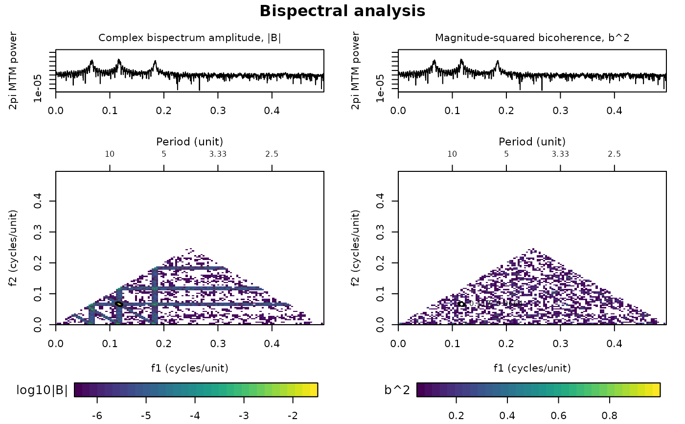
The bispectral_analysis function estimates the complex bispectrum \(B(f_1,f_2) = mean[X(f_1) X(f_2) conj(X(f_1+f_2))]\), the biphase \(arg B\) and the Kim and Powers (1979) magnitude-squared bicoherence (bounded in [0,1]) of an evenly or unevenly sampled series. Two estimators are available: a direct FFT bispectrum averaged over tapered (WOSA/Welch) segments, and a two-dimensional hexagonal frequency-smoothed direct estimate on the native DFT grid. The numerical domain is the non-redundant positive principal domain (\(k_2 \le k_1\), \(k_1+k_2\) below Nyquist). Before estimation the series is cleaned (non-finite rows removed, sorted, duplicate coordinates averaged), regularised by interpolation when the sampling is irregular, detrended and optionally standardised. Optional inference: an analytical Beta(1,R-1) pointwise reference, pointwise Monte Carlo surrogate thresholds, or a global maximum-statistic surrogate test (family-wise error control over the full computed principal domain) using Fourier-transform (FT) phase-randomised or IAAFT surrogates (Schreiber and Schmitz, 1996) with plus-one Monte Carlo p-values. High bicoherence indicates repeatable quadratic phase coupling at \((f_1,f_2,f_1+f_2)\); it is not by itself evidence of causality or energy transfer. Translated from Acycle v3.1 bispectralAnalyze.m, bispectralDefaults.m, bispectralPreprocess.m, bispectralEstimate.m and bispectralSignificance.m (Mingsong Li).

Usage

bispectral_analysis(
  data = NULL,
  estimator = NULL,
  n_segments = NULL,
  overlap = 50,
  window = "hann",
  segment_detrend = "mean",
  smoothing_span = 3,
  smoothing_kernel = "daniell",
  detrend = "linear",
  poly_order = 2,
  standardize = TRUE,
  interpolate = "auto",
  interp_method = "linear",
  sample_interval = NULL,
  irregular_tol = 0.01,
  gap_warning_factor = 5,
  input_policy = "prepare",
  nfft = NULL,
  zero_pad = 1,
  max_freq_bins = 512,
  significance = "none",
  conf_level = 0.95,
  n_sim = 999,
  surrogate_type = "iaaft",
  iaaft_iter = 200,
  iaaft_tol = 0.02,
  max_attempts = NULL,
  seed = NULL,
  genplot = FALSE,
  verbose = FALSE,
  standardise = NULL
)

Arguments

data: Series to analyse (numeric matrix or data frame with at least two columns: depth or time in column 1, proxy value in column 2; further columns are ignored). At least 32 finite observations with distinct coordinates are needed; even or uneven sampling (see interpolate). Required, no default (Default=NULL gives an error).
estimator: Bispectrum estimator (character): "wosa" (direct FFT bispectrum averaged over tapered, overlapping segments; also "welch") or "frequency-smoothed" (direct estimate on the native DFT grid smoothed with a hexagonal kernel). NULL chooses as Acycle does: "wosa", unless three 32-point segments do not fit, then "frequency-smoothed". Default=NULL.
n_segments: Number of WOSA segments (integer, >= 3); more segments give a more stable estimate with a coarser frequency resolution. NULL uses min(8, maximum number of 32-point segments) as in Acycle. Default=NULL.
overlap: Overlap of adjacent WOSA segments in percent (numeric, 0 <= overlap < 90). Default=50.
window: Taper applied to every segment (character): "hann", "hamming", "blackman" or "rectangular" (no taper). Default="hann".
segment_detrend: Detrending applied to each segment (or to the whole record for the frequency-smoothed estimator) before the FFT (character): "none", "mean" or "linear". Default="mean".
smoothing_span: Span of the hexagonal frequency-smoothing kernel of the frequency-smoothed estimator (odd integer, >= 3; 3 averages 7 triads); larger spans give a smoother, lower-resolution estimate. Default=3.
smoothing_kernel: Weights of the hexagonal smoothing kernel (character): "daniell" (uniform) or "cosine" (raised cosine). Default="daniell".
detrend: Detrending of the whole record before the estimation (character): "none", "mean", "linear" or "polynomial" (order poly_order). Default="linear".
poly_order: Order of the polynomial removed when detrend = "polynomial" (integer, 1 to 10 and below N - 1). Default=2.
standardize: Standardise the series to zero mean and unit standard deviation after detrending (logical, TRUE or FALSE). Default=TRUE.
interpolate: When the series is interpolated onto a regular grid (character): "auto" only when the sampling is irregular (see irregular_tol), "always", or "never" (an irregular series then gives an error). Default="auto".
interp_method: Interpolation method for the regular grid (character): "linear", "pchip" (shape-preserving piecewise cubic) or "makima" (modified Akima). Default="linear".
sample_interval: Sample interval of the regular grid, in the unit of the first column of data (numeric, > 0, not coarser than the median original spacing); NULL uses the median original spacing. Default=NULL.
irregular_tol: Largest relative departure of the sample spacing from the grid interval that is still treated as regular sampling, used with input_policy = "prepare" (numeric, >= 0). Default=0.01.
gap_warning_factor: Largest original gap, in sample intervals, above which a warning about interpolation across gaps is stored in the result (numeric, > 0). Default=5.
input_policy: How irregular input is handled (character): "prepare" cleans the input (removes non-finite rows, sorts, averages duplicate coordinates) or "strict" refuses non-finite, unsorted or duplicated rows with an error. Default="prepare".
nfft: FFT length of every WOSA segment (positive integer); NULL uses round(segment length x zero_pad). Ignored by the frequency-smoothed estimator. Default=NULL.
zero_pad: Zero-padding factor of the WOSA segments, used when nfft = NULL (numeric, > 0). Default=1.
max_freq_bins: Maximum number of frequency bins computed along each frequency axis (integer, >= 16); larger grids are decimated with a constant stride to limit computing time and memory. Default=512.
significance: Type of inference on the bicoherence (character): "none", "analytical" (Beta(1, R - 1) pointwise reference), "pointwise" (pointwise surrogate thresholds) or "global" (maximum-statistic surrogate test with family-wise error control over the computed principal domain). Default="none".
conf_level: Confidence level of the significance threshold (numeric, strictly between 0.5 and 1). Default=0.95.
n_sim: Number of accepted surrogates for significance = "pointwise" or "global" (integer, 19 to 99999, and large enough to reach 1 - conf_level). Default=999.
surrogate_type: Type of surrogate (character): "iaaft" (iterative amplitude-adjusted Fourier transform, keeps both spectrum and amplitude distribution) or "ft" (Fourier phase randomisation). Default="iaaft".
iaaft_iter: Maximum number of IAAFT iterations per surrogate (positive integer). Default=200.
iaaft_tol: Largest accepted relative Fourier-amplitude error of an IAAFT surrogate (non-DC, non-Nyquist bins); worse surrogates are rejected and replaced (numeric, 0 < iaaft_tol <= 1). Default=0.02.
max_attempts: Maximum number of surrogate attempts, including rejected ones (integer, >= n_sim); NULL allows n_sim + max(10, ceiling(0.1 n_sim)). Default=NULL.
seed: Seed of the random number generator (integer), so that the surrogates can be reproduced; NULL leaves the current random state unchanged. Default=NULL.
genplot: Plot the result with plot_bispectral (logical, TRUE or FALSE). Default=FALSE.
verbose: Print progress messages and a progress bar for the surrogates (logical, TRUE or FALSE). Default=FALSE.
standardise: British spelling of standardize; if given it overrides standardize. Default=NULL.

Value

A list with elements frequency (computed frequency axis, cycles per unit), bispectrum (complex matrix; rows = f2, columns = f1; NA outside the principal domain), bispectrum_magnitude, biphase (radians, NA where undefined), bicoherence_squared, denominator, valid_mask, principal_domain_mask, power (segment- averaged power on the frequency axis), pair_index, pair_bicoherence_squared, meta (estimator settings and diagnostics), processed_data (2-column processed series), preprocessing (list), significance (list with method, threshold, threshold_matrix, p_value, significant_mask, surrogate_maxima, surrogate_spectral_errors, attempt/rejection counts and warnings), significant_mask and warnings.

References

Kim, Y.C., Powers, E.J., 1979. Digital bispectral analysis and its applications to nonlinear wave interactions. IEEE Transactions on Plasma Science 7, 120-131.

Choudhury, M.A.A.S., Shah, S.L., Thornhill, N.F., 2008. Diagnosis of Process Nonlinearities and Valve Stiction. Springer.

Schreiber, T., Schmitz, A., 1996. Improved surrogate data for nonlinearity tests. Physical Review Letters 77, 635-638.

Li, M., Hinnov, L., Kump, L., 2019. Acycle: Time-series analysis software for paleoclimate research and education. Computers & Geosciences 127, 12-22.

Author

Michiel Arts (R translation); original MATLAB code: Mingsong Li (Acycle bispectral module).

Examples

# \donttest{
# quadratic phase coupling: f3 = f1 + f2 with phase3 = phase1 + phase2 + 0.4
set.seed(1)
seg_len <- 256
n_seg <- 16
t <- 0:(seg_len * n_seg - 1)
y <- numeric(length(t))
f1 <- 30 / seg_len
f2 <- 17 / seg_len
for (s in seq_len(n_seg)){
  idx <- (s - 1) * seg_len + seq_len(seg_len)
  p1 <- 2 * pi * runif(1)
  p2 <- 2 * pi * runif(1)
  y[idx] <- cos(2 * pi * f1 * t[idx] + p1) +
    0.85 * cos(2 * pi * f2 * t[idx] + p2) +
    0.65 * cos(2 * pi * (f1 + f2) * t[idx] + p1 + p2 + 0.4) +
    0.18 * rnorm(seg_len)
}
res <- bispectral_analysis(data = cbind(t, y), n_segments = 16,
  overlap = 0, detrend = "none", max_freq_bins = 256,
  significance = "global", n_sim = 19, seed = 1, genplot = TRUE)

# }