Getting started with WaverideR

WaverideR extracts cyclic signals from stratigraphic and other time series with the continuous wavelet transform and the superlet transform. This vignette follows a typical cyclostratigraphic workflow on the magnetic susceptibility record of the Sullivan core (mag, Pas et al., 2018): transform, test, estimate the sedimentation rate and read off the uncertainty. The records are shortened and the resolution is reduced so that the vignette runs in a few seconds; use the full records and finer settings (smaller dj, more simulations) for real work.

1. Wavelet transform

analyse_wavelet() takes a two-column table (depth or time, value). The record is interpolated to its median spacing, padded, and transformed with a Morlet wavelet. omega_nr is the central angular frequency of the Morlet wavelet: a larger value gives a better resolution in period and a poorer resolution in depth.

mag_short <- mag[1:300, ]
wt <- analyse_wavelet(data = mag_short, dj = 1/12, lowerPeriod = 0.2, upperPeriod = 32,
                      verbose = FALSE, omega_nr = 8)
plot_wavelet(wt, periodlab = "Period (m)", x_lab = "depth (m)", add_avg = TRUE)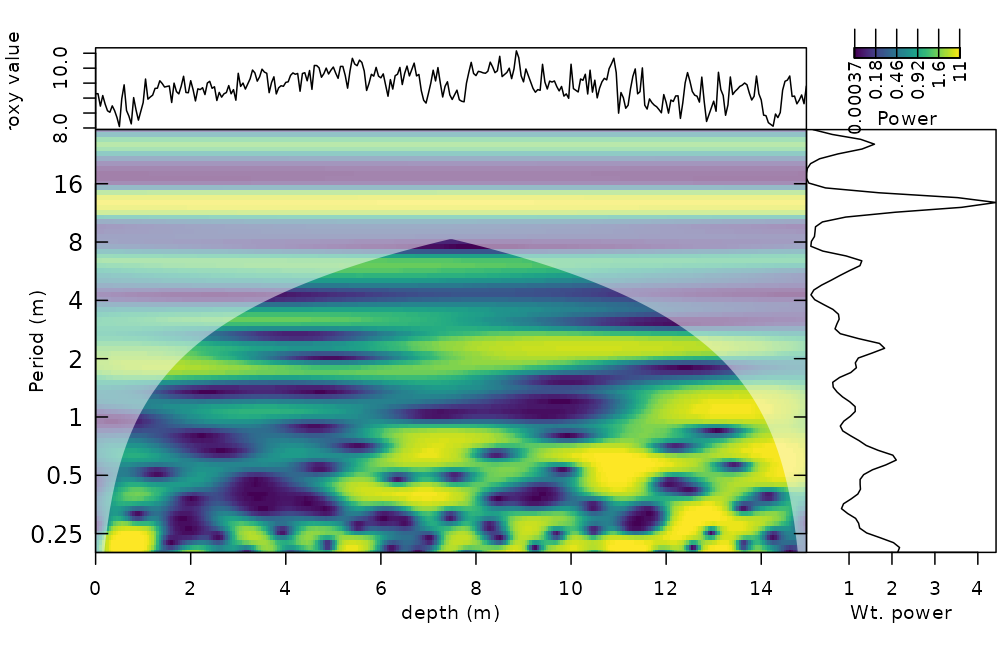

The shaded area outside the dome-shaped boundary is the cone of influence, where edge effects matter.

2. Is a peak significant?

wavelet_significance() outlines the cells of the scalogram that are significant against a red noise (AR(1)) background (Torrence and Compo, 1998) and gives the level of the global spectrum. method = "surrogate" does the same with noise surrogates that pass through the same transform, and works for superlets too.

sig <- wavelet_significance(wt)
plot_wavelet(wt, periodlab = "Period (m)", x_lab = "depth (m)", add_avg = TRUE, add_signif = sig)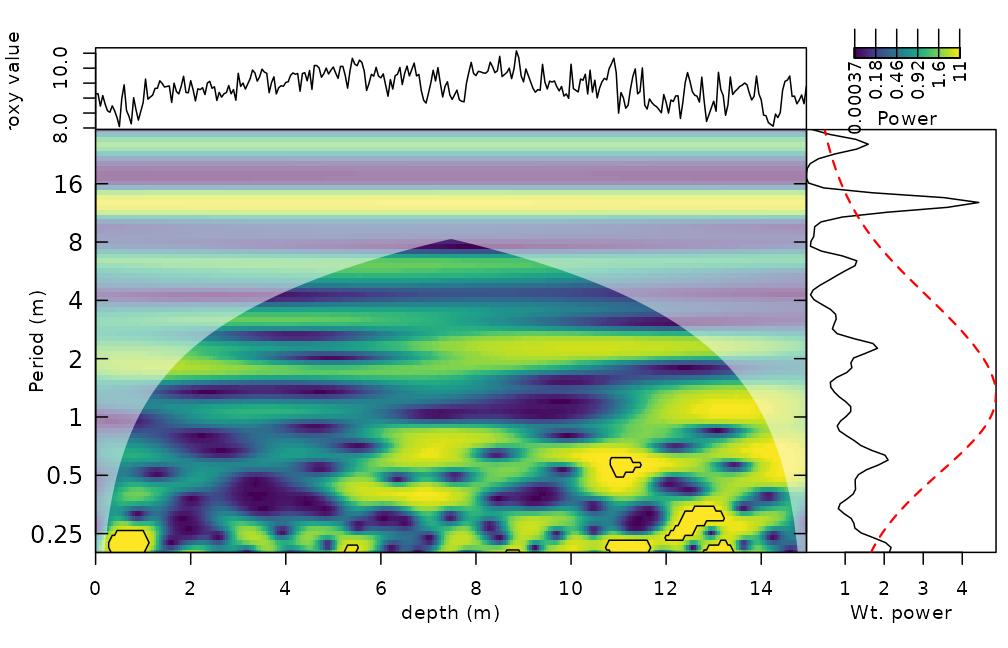

To test the power in a band, for example the precession band, use the scale-averaged significance. It is valid for any omega_nr, because the null distribution is derived from the wavelet itself rather than from a fixed constant:

band <- wavelet_band_significance(wt, period_range = c(0.8, 1.6), background = "ar1")
band
#> Significance of scale-averaged wavelet power (exact, ar1 background, level 0.95)
#>   band: periods 0.8476 to 1.6 (12 scales)
#>   equivalent degrees of freedom: 5.06 
#>   expected band average under the null: 0.2147   critical value: 0.478 
#>   significant points: 0 of 242 outside the cone of influence
plot(band)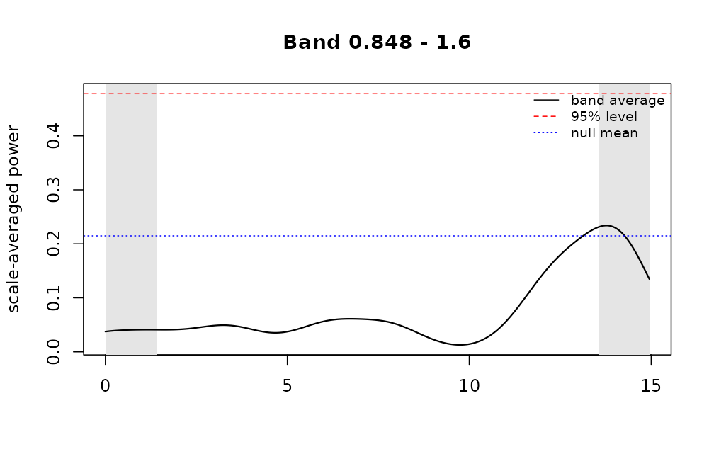

3. Superlets

Superlets combine several wavelet widths at every frequency and give a better resolution in both period and depth. The order grows from o[1] at the lowest to o[2] at the highest frequency. With mult = TRUE the i-th wavelet has i * c1 cycles, with mult = FALSE it has c1 + i - 1 cycles (Moca et al., 2021).

sl <- analyse_superlet(mag_short, upperPeriod = 32, lowerPeriod = 0.4, Nf = 60,
                       c1 = 3, o = c(1, 4), mult = TRUE)
plot_superlet(sl, periodlab = "Period (m)", x_lab = "depth (m)")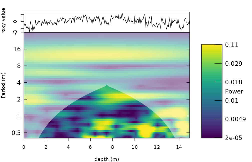

4. Sedimentation rate from the wavelet spectrum

flmw() tests, for every depth and every trial sedimentation rate, how well the expected astronomical periods (in kyr) match the peaks of the wavelet spectrum. flmw_path() adds continuity along depth.

cycles <- c(2376, 1600, 1180, 696, 406, 110)   # periods in kyr
sr <- flmw(wavelet = wt, sedrate_low = 0.5, sedrate_high = 4, spacing = 0.5,
           cycles = cycles, x_lab = "depth", y_lab = "sedrate", run_random = FALSE,
           genplot = FALSE, plot_res = 2)
str(sr, max.level = 1)
#> List of 13
#>  $ slope_coeff_mat      : num [1:8, 1:300] 0.0914 0.1127 0.0654 0.1211 0.2011 ...
#>  $ corr_coeff_mat       : num [1:8, 1:300] 0.995 0.998 0.994 0.987 0.97 ...
#>  $ nr_compenents_mat    : num [1:8, 1:300] 5 5 4 4 3 3 3 3 5 5 ...
#>  $ orig_mat             : num [1:8, 1:300] 0.7378 0.0698 0.6328 -0.6982 -1.4504 ...
#>  $ slope_coeff_mat_per  : num [1:8, 1:300] NA NA NA NA NA NA NA NA NA NA ...
#>  $ corr_coeff_mat_per   : num [1:8, 1:300] NA NA NA NA NA NA NA NA NA NA ...
#>  $ nr_compenents_mat_per: num [1:8, 1:300] NA NA NA NA NA NA NA NA NA NA ...
#>  $ orig_mat_per         : num [1:8, 1:300] NA NA NA NA NA NA NA NA NA NA ...
#>  $ depth                : num [1:300] 0 0.05 0.1 0.15 0.2 ...
#>  $ y_axis               : num [1:8] 0.5 1 1.5 2 2.5 3 3.5 4
#>  $ score_mat            : num [1:8, 1:300] 0.754 0.738 0.619 0.578 0.387 ...
#>  $ best_sedrate         : num [1:300] 0.5 0.5 0.5 0.5 0.5 0.5 0.5 0.5 0.5 0.5 ...
#>  $ method               : chr "classic"

The alternative is to sum the spectral power above a red-noise threshold. The red noise is simulated with the autocorrelation, mean and variance of the record (model_red_noise_wt()), and sum_power_sedrate() then scores each trial sedimentation rate (use many more simulations in practice):

set.seed(1)
rn <- model_red_noise_wt(wt, n_simulations = 10)
ssr <- sum_power_sedrate(red_noise = rn, wavelet = wt, percentile = 0.75,
                         sedrate_low = 0.5, sedrate_high = 4, spacing = 0.5, cycles = cycles)
dim(ssr$power_max_mat)   # trial sedimentation rates x depths
#> [1]   8 300

5. Uncertainty of the frequency

The Morlet wavelet has a limited frequency resolution; wavelet_uncertainty() gives the conservative analytical uncertainty for the omega_nr used, which is the input for the uncertainty of age models built from tracked periods.

6. Parallel computing and memory

Everything is sequential by default. Set run_multicore = TRUE (and optionally n_cores) in the functions that offer it, or options(waverider.n_cores = 2). The number of cores is capped by the physical cores, the free memory and the CRAN limit, and results do not depend on it.

References

Moca, V.V., Barbulescu, A., Nagy-Dabacan, A., Muresan, R.C. (2021). Time-frequency super-resolution with superlets. Nature Communications 12, 337.

Pas, D., Hinnov, L., Day, J.E., Kodama, K., Sinnesael, M., Liu, W. (2018). Cyclostratigraphic calibration of the Famennian stage (Late Devonian, Illinois Basin, USA). Earth and Planetary Science Letters 488, 102-114.

Torrence, C. and Compo, G.P. (1998). A practical guide to wavelet analysis. Bulletin of the American Meteorological Society 79, 61-78.