Gaussian band-pass filter (Acycle)

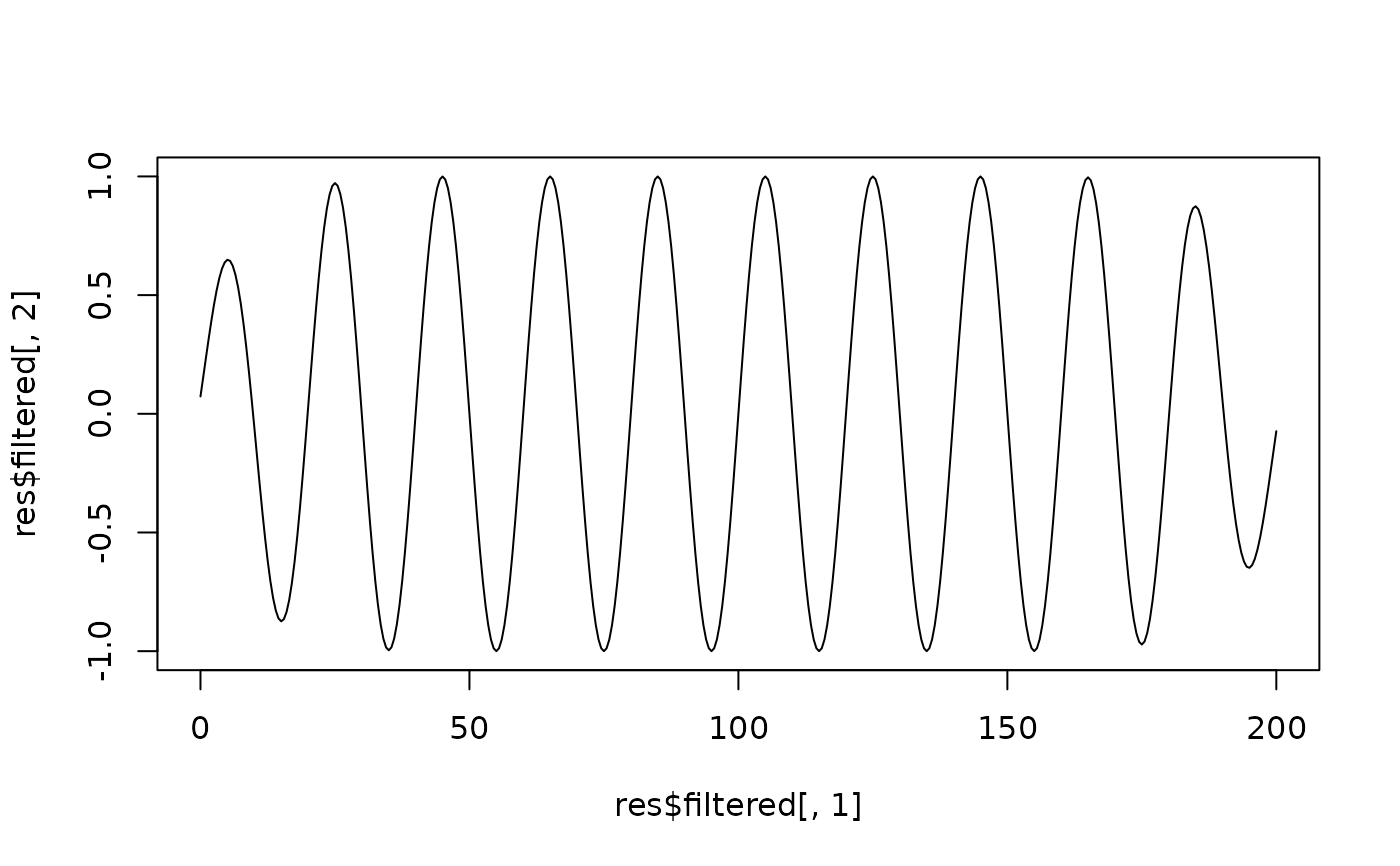
The gaussian_bandpass function applies the Acycle Gaussian band-pass filter to a regularly sampled series. The value mean is removed, the series is zero padded to 10 * 2^nextpow2(n) samples and multiplied in the Fourier domain by a symmetric Gaussian response centred on (f_low + f_high) / 2 whose lower and upper frequencies are exact half-power (-3 dB, gain 1/sqrt(2)) points. The amplitude envelope is the modulus of the analytic signal (MATLAB hilbert) of the filtered series. The Gaussian parameterisation mimics the Gaussian filter of Analyseries 2.0 (Paillard et al., 1996), as implemented by K. Ramamurthy (2013) and corrected by L. Hinnov (2016). Translated from Acycle v3.1 acycleBandpassFilter.m (method "gaussian") and gaussfilter.m (Mingsong Li).

Usage

gaussian_bandpass(
  data = NULL,
  f_low = NULL,
  f_high = NULL,
  genplot = FALSE,
  x_lab = "depth",
  y_lab = "proxy"
)

Arguments

data

Numeric two-column matrix or data frame: depth/time in column 1 (strictly increasing and regularly sampled, relative spacing tolerance 1e-5; interpolate first if needed) and the proxy value in column 2; at least eight rows, all values finite. Required (Default=NULL).

f_low

Lower half-power (-3 dB) frequency of the pass band, in cycles per unit of the depth/time column (numeric, > 0; e.g. 1/25 to keep periods shorter than 25 m). Required (Default=NULL).

f_high

Upper half-power (-3 dB) frequency of the pass band, in cycles per unit of the depth/time column (numeric, > f_low and strictly below the Nyquist frequency 1 / (2 * sampling interval)). Required (Default=NULL).

genplot

Plot the demeaned data with the filtered signal and its envelope, and the filter response (logical, TRUE or FALSE). Default=FALSE.

x_lab

Label of the x-axis of the data plot (character). Default="depth".

y_lab

Label of the y-axis of the data plot (character). Default="proxy".

Value

A list with elements

filtered

matrix with columns depth, filtered and envelope.

response

matrix with columns frequency and gain: the one-sided Gaussian response (0 to Nyquist of the padded FFT grid).

f_low, f_high, f_centre

the pass band used.

sample_interval

median sample spacing.

nyquist

Nyquist frequency 1 / (2 * sample_interval).

nfft

length of the zero-padded FFT.

input_mean

mean removed before filtering.

References

Li, M., Hinnov, L., Kump, L., 2019. Acycle: Time-series analysis software for paleoclimate research and education. Computers & Geosciences 127, 12-22. <doi:10.1016/j.cageo.2019.02.011>

Paillard, D., Labeyrie, L., Yiou, P., 1996. Macintosh program performs time-series analysis. Eos 77, 379. <doi:10.1029/96EO00259>

Author

Michiel Arts (R translation); original MATLAB code: Mingsong Li (Acycle), Linda Hinnov and K. Ramamurthy (gaussfilter).

Examples

# \donttest{
depth <- seq(0, 200, by = 0.5)
proxy <- sin(2 * pi * depth / 20) + 0.5 * sin(2 * pi * depth / 5)
res <- gaussian_bandpass(data = cbind(depth, proxy), f_low = 0.04,
  f_high = 0.06, genplot = FALSE)
plot(res$filtered[, 1], res$filtered[, 2], type = "l")

# }