Plot an adaptive multitaper spectrum with background and detections
Source:R/plot_amtm_spectrum.R
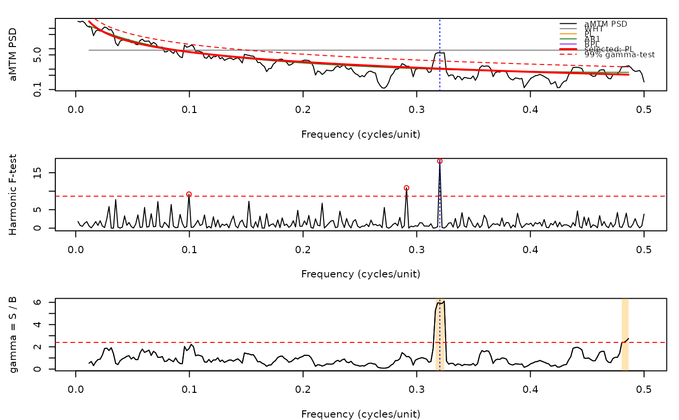
plot_amtm_spectrum.RdThe plot_amtm_spectrum function plots the output of
amtm_spectrum: (top) the aMTM PSD with all fitted background models,
the selected model and its gamma-test threshold; (middle) the harmonic F-test with
its threshold; (bottom) the gamma statistic S/B with its threshold and the gamma
bands. Detected periodic signals are marked with vertical lines. The frequency axis
is in cycles per unit of the input depth/time column. Translated/adapted from the
plotting code of the amtm_signaldetect tutorial notebook (Hector A. Salinas).
Usage
plot_amtm_spectrum(
  amtm = NULL,
  xlim = NULL,
  log_freq = FALSE,
  freq_lab = "Frequency (cycles/unit)",
  show_all_models = TRUE
)
Arguments
- amtm
Adaptive multitaper result to plot: the list returned by
amtm_spectrum. Required (Default=NULLgives an error).- xlim
Frequency range shown in all three panels, in cycles per unit of the input depth/time column (numeric vector of length 2,
c(min, max)).NULLshows all positive frequencies.Default=NULL.- log_freq
Use a logarithmic frequency axis in all panels (logical, TRUE or FALSE); the PSD axis of the top panel is always logarithmic.
Default=FALSE.- freq_lab
Label of the frequency axis (character).
Default="Frequency (cycles/unit)".- show_all_models
Draw every fitted background model (white noise
WHT, power lawPL,AR1, bending power lawBPL) in the top panel in addition to the selected model (logical); withFALSEonly the selected model and its gamma-test threshold are drawn.Default=TRUE.
References
Di Matteo, S., Viall, N. M., & Kepko, L. (2021). Journal of Geophysical Research: Space Physics, 126, e2020JA028748. doi:10.1029/2020JA028748
Examples
# \donttest{
set.seed(2)
n <- 512
t <- 0:(n - 1)
x <- as.numeric(stats::filter(rnorm(n), 0.9, method = "recursive")) +
0.5 * sin(2 * pi * 0.1 * t) + 0.3 * sin(2 * pi * 0.32 * t)
res <- amtm_spectrum(data = cbind(t, x))
plot_amtm_spectrum(res)
 # }