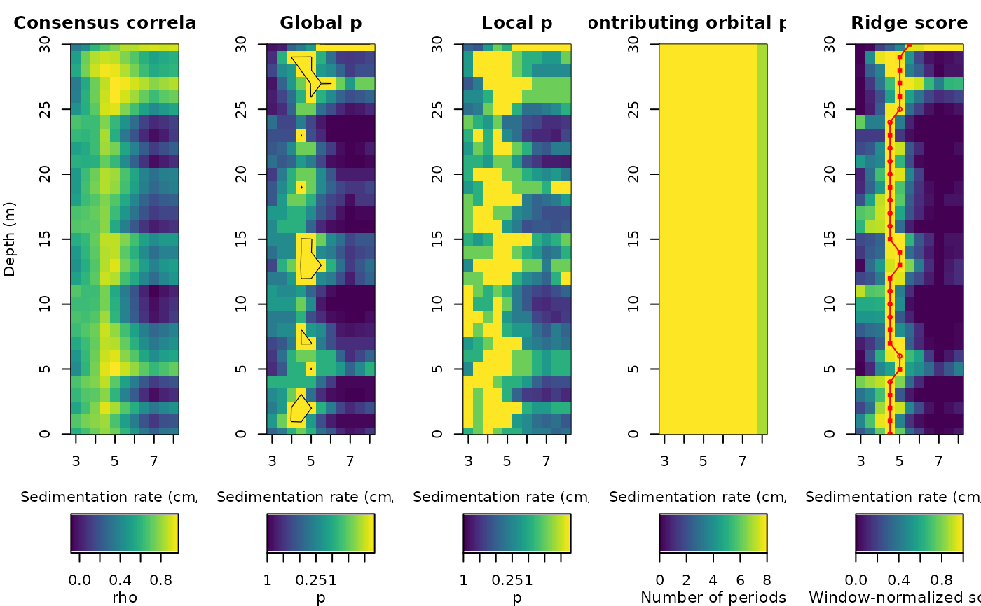
Plot Blocked / Interleaved eCOCO maps — plot_ecoco

Plots the five eCOCO maps used by Acycle for Blocked and Interleaved eCOCO: consensus correlation, consensus SR-global p and same-rate local p (both as -log10(p) with their own 1-2-5 display range, limited by the Monte Carlo resolution 1/(n_sim+1), with the 0.05 and 0.01 contours), the number of contributing orbital periods, and the window-normalised ridge score with the tracked ridge (filled squares: global p <= 0.05; filled circles: local p <= 0.01; open circles: neither). Also accepts cocoR ecoco_adaptive results. Translated from Acycle v3.1 ecocoplot.m (Mingsong Li); base graphics only.

Usage

plot_ecoco_cv(
  ecoco = NULL,
  panels = 1:5,
  reverse_depth = FALSE,
  palette = .wr_hcl_cols(64, "viridis")
)

Arguments

ecoco: eCOCO result to plot: the list returned by ecoco_blocked, ecoco_interleaved or ecoco_adaptive (with sr, depth, rho, p_global, p_local, norbit, score and track). Required (Default=NULL gives an error).
panels: Which maps to draw, side by side in the order given (integer vector with values 1 to 5): 1 consensus correlation coefficient (rho), 2 SR-global p, 3 same-rate local p, 4 number of contributing orbital periods, 5 window-normalised ridge score with the tracked ridge. Default=1:5.
reverse_depth: Reverse the depth axis so that depth increases downwards (logical, TRUE or FALSE). Default=FALSE.
palette: Colours of the colour scale of all maps (character vector of colours, e.g. the output of hcl.colors); the first colour is used for the lowest values and the length of the vector sets the number of colour levels. Default= 64 viridis colours (dark purple to yellow).

Value

Invisibly, the list of plotted matrices (rho, -log10 p maps, orbit count, normalised score) and the ridge.

References

Li, M., Kump, L.R., Hinnov, L.A., Mann, M.E., 2018. Tracking variable sedimentation rates and astronomical forcing in Phanerozoic paleoclimate proxy series with evolutionary correlation coefficients and hypothesis testing. Earth and Planetary Science Letters 501, 165-179.

Author

Michiel Arts (R translation); original MATLAB code: Mingsong Li

Examples

# \donttest{
set.seed(2)
dt <- 0.05
depth <- seq(0, 30, by = dt)
tt <- depth * 100 / 5
x <- sin(2 * pi * tt / 405.7) + 0.8 * sin(2 * pi * tt / 98.9) +
  0.5 * sin(2 * pi * tt / 40.99) + 0.4 * sin(2 * pi * tt / 23.68) +
  0.3 * rnorm(length(tt))
res <- ecoco_blocked(cbind(depth, x), window = 10, sr = seq(3, 8, 0.5),
                     step_depth = 1, pad = 400, n_sim = 20)
#> Warning: Blocked eCOCO has no tested rate with complete all-nine training geometry; continuing with the partial-orbit target at 8 of 11 rates (degraded/exploratory result).
plot_ecoco_cv(res)

# }