Plot superlet scalogram using the outcome of the analyse_superlet function.
Usage
plot_superlet(
  superlet = NULL,
  lowerPeriod = NULL,
  upperPeriod = NULL,
  n.levels = 100,
  palette_name = "viridis",
  color_brewer = "viridis",
  useRaster = TRUE,
  periodlab = "Period (metres)",
  x_lab = "depth (metres)",
  keep_editable = FALSE,
  dev_new = wr_dev_new_default(),
  plot_dir = TRUE,
  add_lines = NULL,
  add_points = NULL,
  add_abline_h = NULL,
  add_abline_v = NULL,
  add_data = TRUE,
  add_avg = FALSE,
  plot_horizontal = TRUE,
  add_signif = NULL,
  colour_brewer = NULL,
  scale = "auto"
)
Arguments
- superlet
Superlet result to plot: the list returned by
analyse_superlet. Required (Default=NULLgives an error).- lowerPeriod
Shortest period shown on the period axis, in the depth/time unit of the input record (numeric, > 0).
NULLuses the shortest period ofsuperlet.Default=NULL.- upperPeriod
Longest period shown on the period axis, in the depth/time unit of the input record (numeric, >
lowerPeriod).NULLuses the longest period ofsuperlet.Default=NULL.- n.levels
Number of colour levels of the power scale (integer, >= 2); the level breaks are the quantiles of the power, so each colour covers the same share of the scalogram.
Default=100.- palette_name
Name of the colour palette of the power (colour) scale, a character string. Which names are valid depends on
color_brewer:color_brewer = "grDevices":"rainbow","heat.colors","terrain.colors","topo.colors","cm.colors", or any of the 115hcl.colorspalettes (list them withgrDevices::hcl.pals()), for example"viridis","Plasma","Inferno","YlOrRd","Spectral","Blue-Red","Zissou 1".color_brewer = "viridis":"viridis","magma","inferno","plasma","cividis","rocket","mako","turbo".color_brewer = "RColorBrewer":"BrBG","PiYG","PRGn","PuOr","RdBu","RdGy","RdYlBu","RdYlGn","Spectral","Accent","Dark2","Paired","Pastel1","Pastel2","Set1","Set2","Set3","Blues","BuGn","BuPu","GnBu","Greens","Greys","Oranges","OrRd","PuBu","PuBuGn","PuRd","Purples","RdPu","Reds","YlGn","YlGnBu","YlOrBr","YlOrRd"(also listed bywr_brewer_palettes()).color_brewer = "colorRamps":"blue2green","blue2green2red","blue2red","blue2yellow","cyan2yellow","green2red","magenta2green","matlab.like","matlab.like2","ygobb".color_brewer = "scico"(all except"batlowK"need the scico package):"acton","bam","bamako","bamO","batlow","batlowK","batlowW","berlin","bilbao","broc","brocO","buda","bukavu","cork","corkO","davos","devon","fes","glasgow","grayC","hawaii","imola","lajolla","lapaz","lipari","lisbon","managua","navia","nuuk","oleron","oslo","roma","romaO","tofino","tokyo","turku","vanimo","vik","vikO".
Low power is drawn with the first colour of the palette and high power with the last.
Default="viridis".- color_brewer
Palette family from which
palette_nameis taken, a character string:"grDevices","viridis","RColorBrewer","colorRamps"or"scico"(the last one, except for"batlowK", needs the scico package). Seepalette_namefor the palette names of each family.Default="viridis".- useRaster
Draw the scalogram as a raster image (
TRUE) or as vector polygons (FALSE) (logical). WARNING: plotting as a vector image is computationally intensive and gives large files.Default=TRUE.- periodlab
Label of the period axis (character).
Default="Period (metres)".- x_lab
Label of the depth/time axis (character).
Default="depth (metres)".- keep_editable
Keep the plot layout and graphical parameters (
par) after plotting, so that extra elements can be added to the scalogram panel withlines,pointsetc. (logical). WithFALSEthe previousparsettings are restored on exit.Default=FALSE.- dev_new
Open a new plotting window for the plot (logical, TRUE or FALSE). The wavelet plots contain a raster image that needs more room than the small RStudio plot pane, which gives "figure margins too large" errors or clipped text, so a separate window is opened by default in the RStudio GUI. In every other front end (plain R, ESS, Positron, knitr, Rscript) the plot is drawn on the current device and no window is opened. Set TRUE or FALSE to force either behaviour, or set
options(waverider.dev_new = TRUE/FALSE).Default=wr_dev_new_default(): TRUE in the RStudio GUI, FALSE elsewhere.- plot_dir
Direction of the depth/time axis (logical).
TRUEplots increasing depth/time values from left to right (or bottom to top whenplot_horizontal=FALSE);FALSEreverses the axis.Default=TRUE.- add_lines
Lines to draw on the scalogram: a matrix or data frame with depth/time in column 1 and, in each further column, period values (same unit as the period axis) of one line;
NULLdraws none.Default=NULL.- add_points
Points to draw on the scalogram: a matrix or data frame with depth/time in column 1 and, in each further column, period values of one series of points;
NULLdraws none.Default=NULL.- add_abline_h
Numeric vector of positions of horizontal lines, e.g.
c(2, 3, 5, 6): periods whenplot_horizontal=TRUE, depth/time values whenplot_horizontal=FALSE;NULLdraws none.Default=NULL.- add_abline_v
Numeric vector of positions of vertical lines, e.g.
c(2, 3, 5, 6): depth/time values whenplot_horizontal=TRUE(also drawn on the data panel), periods whenplot_horizontal=FALSE;NULLdraws none.Default=NULL.- add_data
Plot the input record in a panel beside the scalogram (logical).
Default=TRUE.- add_avg
Plot the time-averaged superlet power spectrum in a panel beside the scalogram (logical).
Default=FALSE.- plot_horizontal
Orientation of the plot (logical):
TRUEputs depth/time on the x axis and period on the y axis;FALSEputs depth/time on the y axis and period on the x axis.Default=TRUE.- add_signif
Significance result whose significant cells are outlined on the scalogram, and whose critical level of the global spectrum is drawn as a red dashed line on the average power panel: the object returned by
wavelet_significance;NULLdraws no significance.Default=NULL.- colour_brewer
British spelling of
color_brewer, with the same options; if given (notNULL) it overridescolor_brewer.Default=NULL.- scale
Spacing of the colour breaks (character:
"auto","quantile","log","sqrt"or"linear", seeplot_wavelet). In the current version this argument has no effect here: the colour breaks of the superlet scalogram are always then.levelsquantiles of the power.Default="auto".
References
Roesch, A., & Schmidbauer, H. (2018). WaveletComp: Computational Wavelet Analysis. R package version 1.1. https://CRAN.R-project.org/package=WaveletComp
Moca, V. V., Bârzan, H., Nagy-Dăbâcan, A., & Mureșan, R. C. (2021). Time-frequency super-resolution with superlets. Nature Communications, 12(1), 337. doi:10.1038/s41467-020-20539-9
Author
Code based on the "wt.image" functions of the 'WaveletComp' R package Whereas the "analyse_superlet" that generates the input for the plotting function is based on the matlab code in Moca et al. (2021)
Examples
# \donttest{
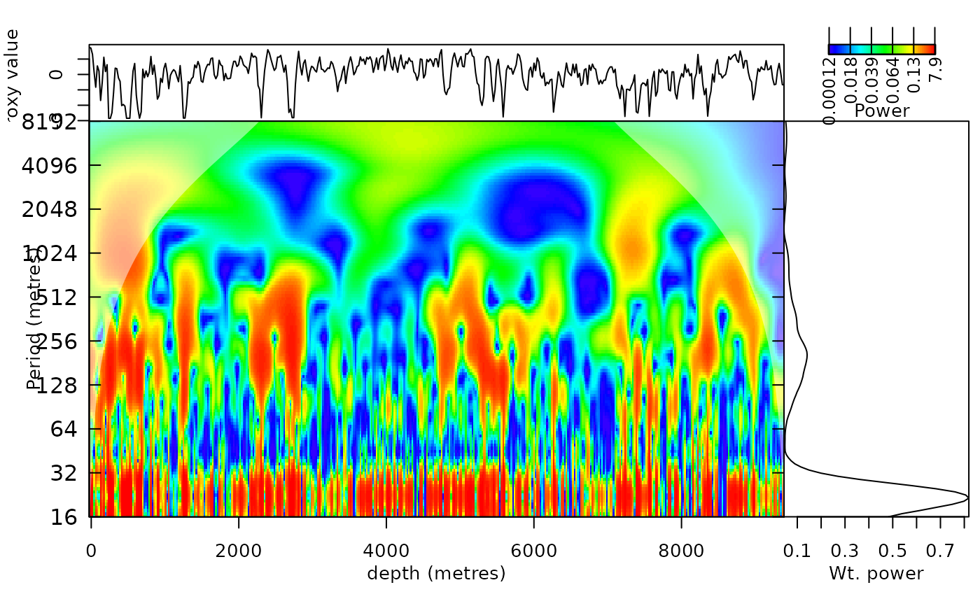
#Example 1. A plot of a wavelet spectra using the Total Solar Irradiance
# data set of Steinhilber et al., (2012)
TSI_super <-
analyse_superlet(
data = TSI,
Nf = 128,
lowerPeriod = 16,
upperPeriod = 8192,
verbose = FALSE,
c1=1,
o = c(1,5),
mult = TRUE)
#> Warning: lowerPeriod is shorter than twice the sampling interval (44): periods below the Nyquist period cannot be resolved
plot_superlet(
superlet = TSI_super,
lowerPeriod = 16,
upperPeriod = 8192,
n.levels = 100,
palette_name = "rainbow",
color_brewer= "grDevices",
useRaster = TRUE,
periodlab = "Period (metres)",
x_lab = "depth (metres)",
keep_editable = FALSE,
dev_new=TRUE,
plot_dir = TRUE,
add_lines = NULL,
add_points= NULL,
add_abline_h = NULL,
add_abline_v = NULL,
add_data = TRUE,
add_avg = TRUE,
plot_horizontal = TRUE)
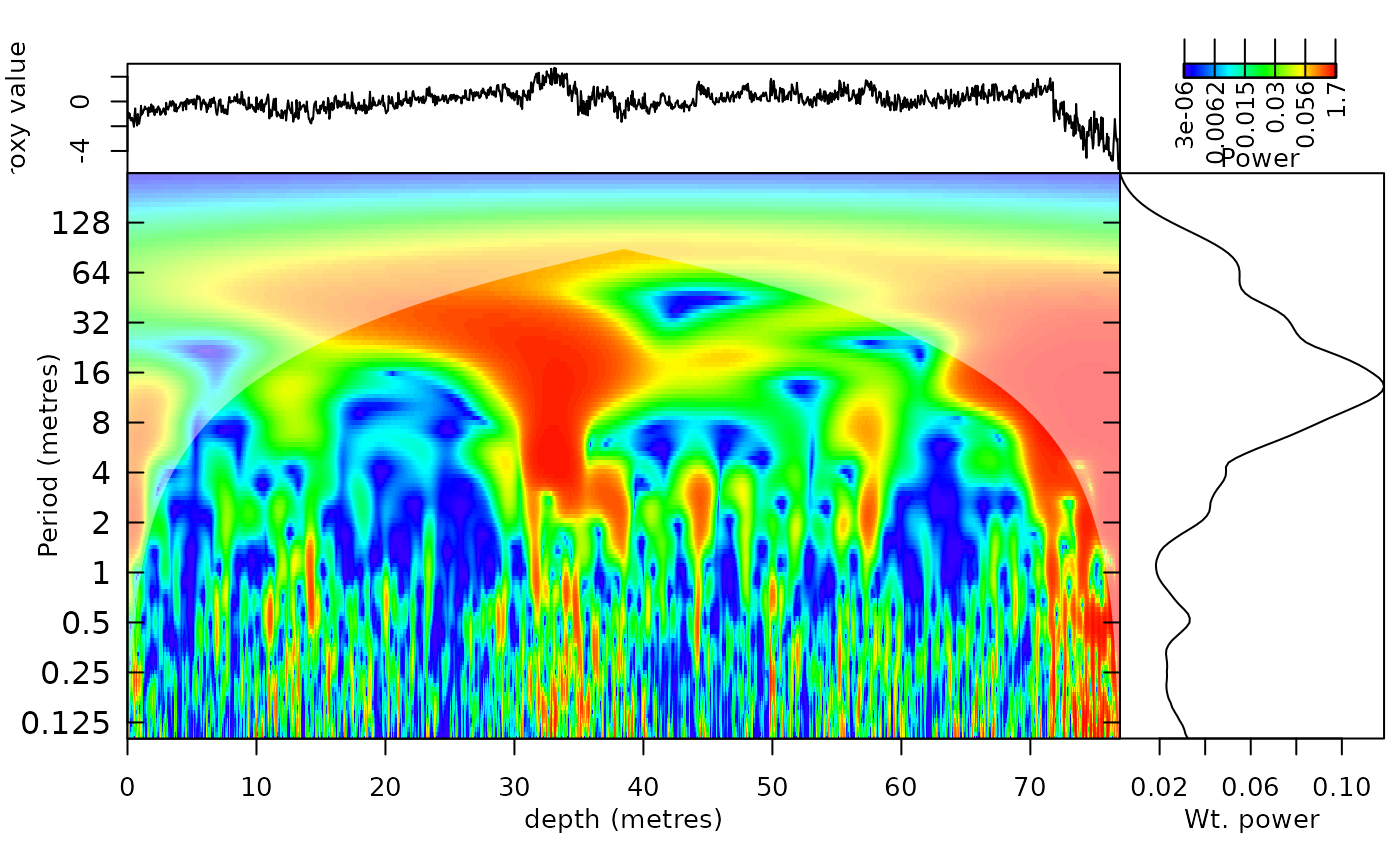
 #Example 2. A plot of a wavelet spectra using the magnetic susceptibility
#data set of Pas et al., (2018)
mag_super <-
analyse_superlet(
data = mag,
Nf = 128,
lowerPeriod = 0.1,
upperPeriod = 254,
verbose = FALSE,
c1=1,
o = c(1,5),
mult = TRUE)
plot_superlet(
superlet = mag_super,
lowerPeriod = 0.1,
upperPeriod = 254,
n.levels = 100,
palette_name = "rainbow",
color_brewer= "grDevices",
useRaster = TRUE,
periodlab = "Period (metres)",
x_lab = "depth (metres)",
keep_editable = FALSE,
dev_new=TRUE,
plot_dir = TRUE,
add_lines = NULL,
add_points= NULL,
add_abline_h = NULL,
add_abline_v = NULL,
add_data = TRUE,
add_avg = TRUE,
plot_horizontal = TRUE)
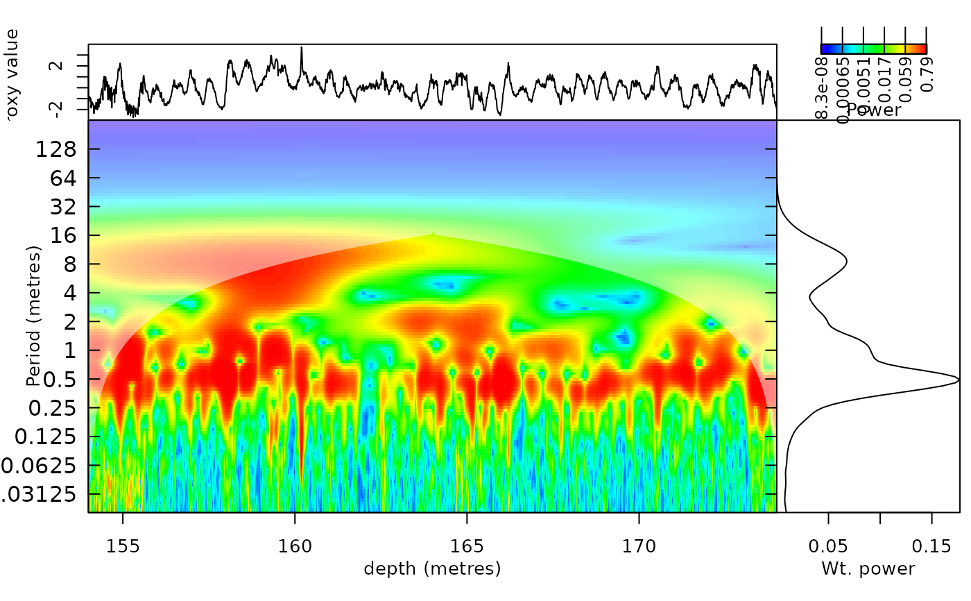
 #Example 3. A plot of a wavelet spectra using the greyscale
# data set of Zeeden et al., (2013)
grey_super <-
analyse_superlet(
data = grey,
Nf = 128,
lowerPeriod = 0.02,
upperPeriod = 256,
verbose = FALSE,
c1=1,
o = c(1,5),
mult = TRUE)
plot_superlet(
superlet = grey_super,
lowerPeriod = 0.02,
upperPeriod = 256,
n.levels = 100,
palette_name = "rainbow",
color_brewer= "grDevices",
useRaster = TRUE,
periodlab = "Period (metres)",
x_lab = "depth (metres)",
keep_editable = FALSE,
dev_new=TRUE,
plot_dir = TRUE,
add_lines = NULL,
add_points= NULL,
add_abline_h = NULL,
add_abline_v = NULL,
add_data = TRUE,
add_avg = TRUE,
plot_horizontal = TRUE)
 # }