Plot windowed fft based spectral analysis results

The plot_win_fft function allows for the (re)plotting of the results of the win_fft

Usage

plot_win_fft(
  win_fft = NULL,
  x_lab = c("depth (m)"),
  y_lab = c("frequency cycle/metre"),
  plot_res = 1,
  perc_vis = 0,
  freq_max = NULL,
  freq_min = NULL,
  keep_editable = FALSE,
  palette_name = "viridis",
  color_brewer = "viridis",
  plot_horizontal = TRUE,
  dev_new = wr_dev_new_default(),
  colour_brewer = NULL
)

Arguments

win_fft

Result of the windowed FFT (required): the list returned by win_fft. Default=NULL.

x_lab

Label of the depth/time axis (character). Default="depth (m)".

y_lab

Label of the frequency axis (character). Default="frequency cycle/metre".

plot_res

Which matrix of win_fft to plot, given as its position in the list (integer, 1 to 9):

1: amplitude (Amplitude_mat),
2: power (Power_mat),
3: phase (Phase_mat),
4: frequency uncertainty (uncer_mat),
5: AR1 confidence level in % (AR1_CL_mat),
6: AR1 red-noise fit (AR1_Fit_mat),
7: AR1 90% confidence power (AR1_90_power_mat),
8: AR1 95% confidence power (AR1_95_power_mat),
9: AR1 99% confidence power (AR1_99_power_mat).

Default=1.

perc_vis

Lower quantile of the colour scale (numeric, between 0 and 1): the colour breaks run from this quantile of the plotted values to the maximum, and values below it are left blank, which hides the background. 0 colours all values. Default=0.

freq_max

Highest frequency plotted, in cycles per depth/time unit (numeric, or NULL for the highest frequency of win_fft). Default=NULL.

freq_min

Lowest frequency plotted, in cycles per depth/time unit (numeric, or NULL for the lowest frequency of win_fft). Default=NULL.

keep_editable

Keep the graphical parameters (par, layout) of the plot after the function returns, so that extra elements can be added to the plot afterwards (logical). With FALSE the previous graphical parameters are restored on exit. Default=FALSE.

palette_name

Name of the colour palette of the power (colour) scale, a character string. Which names are valid depends on color_brewer:

color_brewer = "grDevices": "rainbow", "heat.colors", "terrain.colors", "topo.colors", "cm.colors", or any of the 115 hcl.colors palettes (list them with grDevices::hcl.pals()), for example "viridis", "Plasma", "Inferno", "YlOrRd", "Spectral", "Blue-Red", "Zissou 1".
color_brewer = "viridis": "viridis", "magma", "inferno", "plasma", "cividis", "rocket", "mako", "turbo".
color_brewer = "RColorBrewer": "BrBG", "PiYG", "PRGn", "PuOr", "RdBu", "RdGy", "RdYlBu", "RdYlGn", "Spectral", "Accent", "Dark2", "Paired", "Pastel1", "Pastel2", "Set1", "Set2", "Set3", "Blues", "BuGn", "BuPu", "GnBu", "Greens", "Greys", "Oranges", "OrRd", "PuBu", "PuBuGn", "PuRd", "Purples", "RdPu", "Reds", "YlGn", "YlGnBu", "YlOrBr", "YlOrRd" (also listed by wr_brewer_palettes()).
color_brewer = "colorRamps": "blue2green", "blue2green2red", "blue2red", "blue2yellow", "cyan2yellow", "green2red", "magenta2green", "matlab.like", "matlab.like2", "ygobb".
color_brewer = "scico" (all except "batlowK" need the scico package): "acton", "bam", "bamako", "bamO", "batlow", "batlowK", "batlowW", "berlin", "bilbao", "broc", "brocO", "buda", "bukavu", "cork", "corkO", "davos", "devon", "fes", "glasgow", "grayC", "hawaii", "imola", "lajolla", "lapaz", "lipari", "lisbon", "managua", "navia", "nuuk", "oleron", "oslo", "roma", "romaO", "tofino", "tokyo", "turku", "vanimo", "vik", "vikO".

Low power is drawn with the first colour of the palette and high power with the last. Default="viridis".

color_brewer

Palette family from which palette_name is taken, a character string: "grDevices", "viridis", "RColorBrewer", "colorRamps" or "scico" (the last one, except for "batlowK", needs the scico package). See palette_name for the palette names of each family. Default="viridis".

plot_horizontal

Orientation of the plot (logical): TRUE puts depth/time on the x-axis and frequency on the y-axis, with the mean spectrum to the left; FALSE draws depth/time on the y-axis and frequency on the x-axis, with the mean spectrum on top. Default=TRUE.

dev_new

Open a new plotting window for the plot. The wavelet plots contain a raster image that needs more room than the small RStudio plot pane, which gives "figure margins too large" errors or clipped text, so a separate window is opened by default in the RStudio GUI. In every other front end (plain R, ESS, Positron, knitr, Rscript) the plot is drawn on the current device and no window is opened. Set TRUE or FALSE to force either behaviour, or set options(waverider.dev_new = TRUE/FALSE). Logical. Default=wr_dev_new_default(): TRUE in the RStudio GUI, FALSE elsewhere.

colour_brewer

British spelling of color_brewer, with the same options; if given (not NULL) it overrides color_brewer. Default=NULL.

Value

Returns a plot of, which plot 1 of 8 options, option 1: Amplitude matrix option 2: Power matrix option 3: Phase matrix option 4: AR1_CL matrix option 5: AR1_Fit matrix option 6: AR1_90_power matrix option 7: AR1_95_power matrix option 8: AR1_99_power matrix

Examples

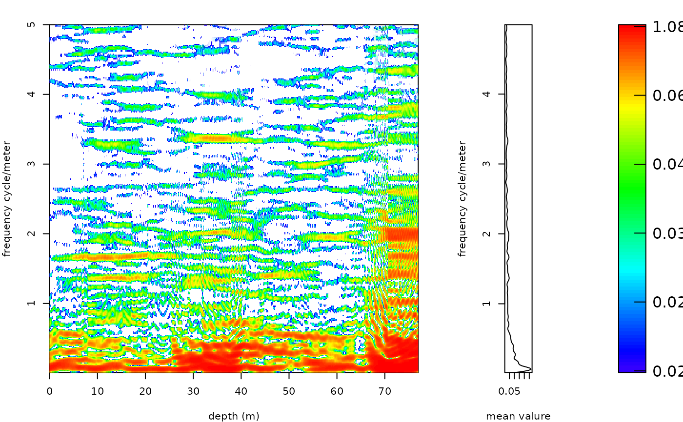
# \donttest{
#Conduct a windowed fft on the magnetic susceptibility record \cr
# of the Sullivan core of Pas et al., (2018).

mag_win_fft <- win_fft(data= mag,
                   padfac = 5,
                   window_size = 12.5,
                   run_multicore = FALSE,
                   genplot = FALSE,
                   palette_name = "rainbow",
                   color_brewer="grDevices",
                   x_lab = c("depth (m)"),
                   y_lab = c("frequency cycle/meter"),
                   plot_res = 1,
                   perc_vis = 0.5,
                   freq_max = 5,
                   freq_min = 0.001,
                   keep_editable=FALSE,
                   verbose=FALSE)

# Plot the amplitude spectra
plot_win_fft(win_fft= mag_win_fft,
x_lab = c("depth (m)"),
y_lab = c("frequency cycle/meter"),
plot_res = 1,
perc_vis = 0.5,
freq_max = 5,
freq_min = 0.001,
keep_editable=FALSE,
palette_name = "rainbow",
color_brewer="grDevices",
plot_horizontal=TRUE,
dev_new=TRUE)


# }