plot the windowed timeOpt sedimentation rate estimation

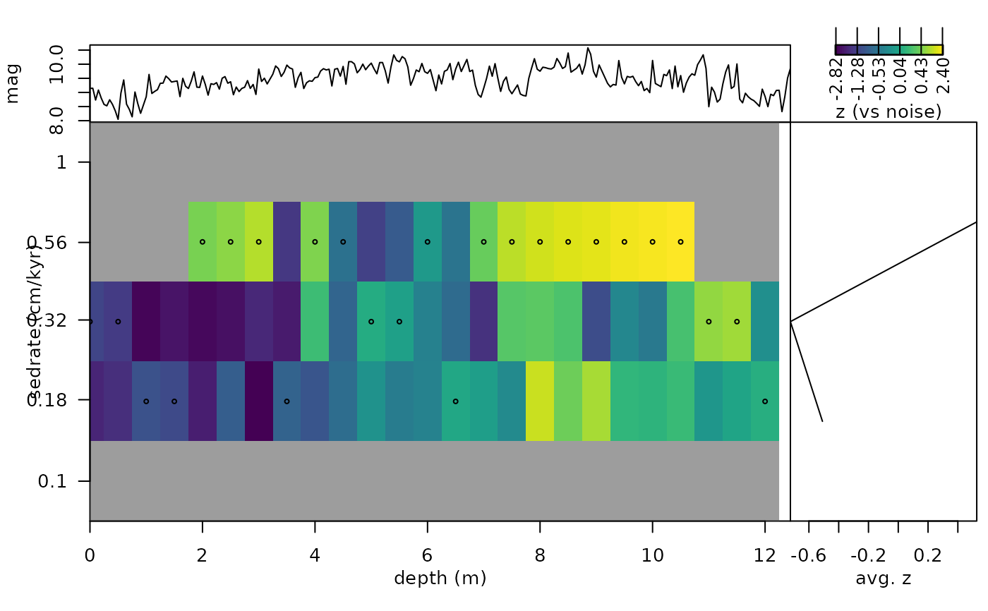
The plot_win_timeOpt function plots a windowed timeOpt sedimentation rate estimation of win_timeOpt.

Usage

plot_win_timeOpt(
  win_timeOpt_result = NULL,
  proxy_name = NULL,
  abline_h = NULL,
  abline_v = NULL,
  add_lines = NULL,
  fig_lts = NULL,
  xlab = "depth (m)",
  ylab = "sedrate (cm/kyr)",
  sel_parameter = 3,
  n.levels = 100,
  corrected = TRUE,
  show_untestable = TRUE,
  show_best = TRUE
)

Arguments

win_timeOpt_result

Result to plot (required): the list returned by win_timeOpt. Default=NULL.

proxy_name

Label of the y-axis of the proxy panel on top (character, e.g. "magnetic susceptibility"); NULL leaves it empty. Default=NULL.

abline_h

Sedimentation rates at which dashed horizontal lines are drawn on the map, in the units of win_timeOpt_result$sedrate (numeric vector, e.g. c(2, 3, 5), or NULL for none). Default=NULL.

abline_v

Depths at which dashed vertical lines are drawn on the map, in the depth unit of the record (numeric vector or NULL for none). Default=NULL.

add_lines

Lines to draw on the map, e.g. a sedimentation rate curve (matrix or data frame, or NULL for none): depth in column 1 and one or more columns of sedimentation rates after it; each column is drawn as a separate line. Default=NULL.

fig_lts

Text (e.g. a figure letter such as "A") written in large type in the upper left corner of the proxy panel (character, or NULL for none). Default=NULL.

xlab

Label of the depth axis (character). Default="depth (m)".

ylab

Label of the sedimentation rate axis (character). Default="sedrate (cm/kyr)".

sel_parameter

Which timeOpt fit to plot (integer): 1 envelope fit, 2 spectral power fit, 3 combined fit (opt). Default=3.

n.levels

Number of colour levels of the map (integer, > 1); the breaks are quantiles of the plotted values. Default=100.

corrected

Plot the bias-corrected z-scores (z_envelope, z_power, z_opt) instead of the raw r-squared values, when the result contains them (bias_correction = "null" in win_timeOpt) (logical). The median z threshold is then drawn as a dotted line on the average panel. Default=TRUE.

show_untestable

Grey out the cells that cannot be tested (too few samples per cycle, too few cycles in the window or window outside the record), as flagged in testable of the result (logical). Default=TRUE.

show_best

Mark the best sedimentation rate of every window (logical); filled symbols are significant at the family-wise level of win_timeOpt, open symbols are not. Default=TRUE.

Value

The output is a plot of a windowed timeOpt with the average curve over all windows.

References

Meyers, S.R. (2019). Cyclostratigraphy and the problem of astrochronologic testing. Earth-Science Reviews 190, 190-223 <doi:10.1016/j.earscirev.2018.11.015>

Author

Based on the eTimeOpt function of the 'astrochron' R package.

Examples

# \donttest{
#plot the windowed timeOpt of the magnetic susceptibility record
#of the Sullivan core of Pas et al., (2018).
set.seed(1)
mag_win_timeOpt <-win_timeOpt(
data = mag[1:250, ],
window_size = 6,
sedmin = 0.1,
sedmax = 1,
numsed = 5,
limit = FALSE,
fit = 2,
fitModPwr = TRUE,
flow = NULL,
fhigh = NULL,
roll = 10 ^ 6,
targetE = c(405.7, 130.7, 123.8, 98.9, 94.9),
targetP = c(20.9, 19.9, 17.1, 17.2),
detrend = TRUE,
normalize =TRUE,
linLog = 1,
bias_correction = "null",
n_null = 6,
noise_model = "ar1",
step = 10,
run_multicore = FALSE,
verbose=FALSE)

plot_win_timeOpt(win_timeOpt_result = mag_win_timeOpt,
proxy_name= "mag",
abline_h=NULL,
abline_v = NULL,
add_lines=NULL,
fig_lts = NULL,
xlab="depth (m)",
ylab= "sedrate (cm/kyr)",
sel_parameter=3,
n.levels=100,
corrected = TRUE)


# }