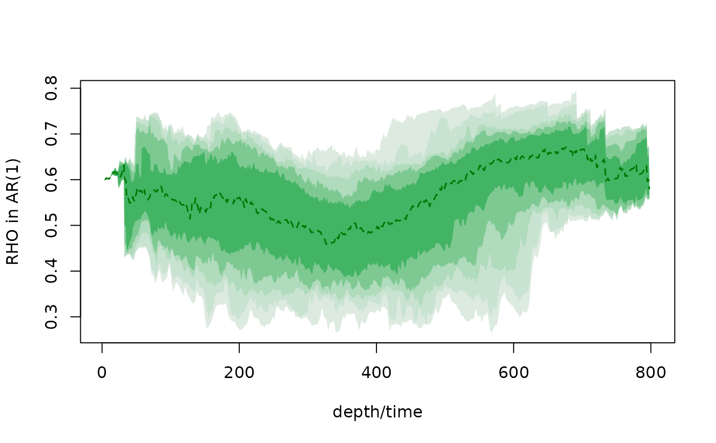
The rho1_evolutive function calculates the
lag-1 autocorrelation coefficient of an AR(1) model in moving windows, as
used in the sedimentary noise model of Li et al. (2018a,b).
With n_sim = 0 a single deterministic run is made
(acycleEvolutionaryRho1.m): the series is linearly interpolated on
a grid anchored at the first coordinate with interval
sample_min, windows of round(window_min/sample_min) points
are linearly detrended and rho1 = sum(z[t] z[t-1]) / sum(z[t-1]^2) of the
demeaned residuals z is reported at the midpoint of each window.
With n_sim > 0 the Acycle Monte Carlo is run (AC.m menu
"Lag-1 autocorrelation coefficient (rho1)"): for every simulation a
sampling interval and a window are drawn uniformly from
[sample_min, sample_max] and [window_min,
window_max], the data are linearly interpolated
(interpolate.m), evolutionary rho1 is computed with
erhoAR1.m (window of round(window/dt) points, linear detrending,
rhoAR1ML.m), window centers are optionally shifted by a random
offset uniform in [-window/2, window/2], and the curves are linearly
interpolated on a regular grid and summarized by the percentiles 2.5, 5,
10, 15.865, 25, 50, 75, 84.135, 90, 95 and 97.5.
Translated from Acycle v3.1 acycleEvolutionaryRho1.m,
acycleInterpolateSeries.m, erhoAR1.m, rhoAR1ML.m, interpolate.m and AC.m
(menu_rho_Callback) (Mingsong Li; rhoAR1 by Dorothee Husson).
Usage
rho1_evolutive(
  data = NULL,
  window_min = NULL,
  window_max = NULL,
  sample_min = NULL,
  sample_max = NULL,
  n_sim = 1000,
  n_out = NULL,
  shift_grid = TRUE,
  seed = NULL,
  verbose = FALSE,
  genplot = FALSE
)
Arguments
- data
Proxy record (required): matrix or data frame with depth/time in column 1 and the proxy value in column 2 (further columns are ignored). Rows with non-finite values are removed and the rows are sorted by depth/time; the depth/time values must be unique.
Default=NULL.- window_min
Window length in depth/time units (numeric, > 0): the window of the single run (
n_sim = 0) or the shortest window drawn in the Monte Carlo run.NULL:min(400, 0.3 * L)where L is the length of the record (in the Monte Carlo run 400 if0.3 * L > 400, otherwise0.3 * L). In the single run the window must span at least three interpolated points.Default=NULL.- window_max
Longest window drawn in the Monte Carlo run, in depth/time units (numeric, >=
window_min); not used whenn_sim = 0.NULL: 500 if0.3 * L > 400, otherwise0.4 * L.Default=NULL.- sample_min
Interpolation interval in depth/time units (numeric, > 0): the interval of the single run or the smallest interval drawn in the Monte Carlo run.
NULLuses the 95th percentile of the sampling intervals ofdata.Default=NULL.- sample_max
Largest interpolation interval drawn in the Monte Carlo run, in depth/time units (numeric, >=
sample_min); not used whenn_sim = 0.NULLuses twice the 95th percentile of the sampling intervals.Default=NULL.- n_sim
Number of Monte Carlo simulations (integer, 0 or >= 50, as in Acycle).
0gives a single deterministic run withwindow_minandsample_min.Default=1000.- n_out
Number of points of the regular depth/time grid on which the Monte Carlo curves are interpolated and summarised (integer, > 1).
NULL:min(1000, number of data points).Default=NULL.- shift_grid
Shift the window centres of every simulation by a random offset, uniform between minus and plus half the window length (logical; Acycle "shift grids" > 1). Only used in the Monte Carlo run.
Default=TRUE.- seed
Seed of the random number generator (integer), so that the Monte Carlo results can be reproduced;
NULLleaves the current random state unchanged.Default=NULL.- verbose
Show a progress bar of the Monte Carlo simulations (logical, TRUE or FALSE).
Default=FALSE.- genplot
Plot the result (logical): the rho1 curve of the single run, or the percentile bands with the median of the Monte Carlo run.
Default=FALSE.
Value
For n_sim = 0 a list with rho1 (matrix [window
center, rho1]), window_points, sample_interval and
window. For the Monte Carlo a list with
percentile (matrix [x, 11 percentiles] on the grid points where
they are defined), median (matrix [x, median]),
percentiles, grid, rho1 (n_out x n_sim matrix of all
realisations) and draws (sampling intervals, windows, shifts).
References
Li, M., Hinnov, L.A., Huang, C., Ogg, J.G., 2018a. Sedimentary noise and sea levels linked to land-ocean water exchange and obliquity forcing. Nature Communications 9, 1004. doi:10.1038/s41467-018-03454-y
Li, M., Huang, C., Hinnov, L., Chen, W., Ogg, J., Tian, W., 2018b. Astrochronology of the Anisian stage (Middle Triassic) at the Guandao reference section, South China. Earth and Planetary Science Letters 482, 591-606. doi:10.1016/j.epsl.2017.11.042
Mudelsee, M., 2002. TAUEST: a computer program for estimating persistence in unevenly spaced weather/climate time series. Computers & Geosciences 28, 69-72.