Sliding-window spectral moments (mean frequency and bandwidth)

The spectral_moments function calculates the first two spectral moments, the mean frequency ($\mu_f$) and the bandwidth ($B$), of a uniformly sampled series in a sliding window (Sinnesael et al., 2018). Because both moments scale with the sedimentation rate, their evolution along a stratigraphic series can be used to detect changes in sedimentation rate.

Within every window the (globally mean-centred) segment is linearly detrended, its one-sided rectangular-window periodogram is computed on an even NFFT grid from DC up to the Nyquist frequency and $$\mu_f = \sum f P(f) / \sum P(f), \quad B = \sqrt{\sum (f-\mu_f)^2 P(f) / \sum P(f)}$$ are calculated.

Two computational paths are available, mirroring the Acycle GUI (SpectralMomentsGUI.m):

the strict deterministic core (default; used whenever sr_mean=NULL and edge_padding is "none" or "zero"). Translated from Acycle v3.1 acycleSpectralMoments.m (Mingsong Li). The window length is rounded (half away from zero) to an integer number of sampling intervals, the step to an integer number of samples, NFFT = pad x window samples (+1 if odd), and window centres are the midpoints of the actual window coordinates.
the legacy path (used when sr_mean is given or when edge_padding is "mirror" or "mean"). Translated from Acycle v3.1 spectralmoments.m and zeropad2.m (Mingsong Li, based on SpectralMoments_with_SR_estimation.m and DetrendSignalPP.m by Matthias Sinnesael). When sr_mean is given the long-term bandwidth trend is estimated with the overlap-add polynomial baseline model of DetrendSignalPP.m (Acycle's 'poly' option) and converted into a relative sedimentation-rate curve scaled to sr_mean ($sr = sr_{mean} B_1 / B_{trend}$, re-centred on sr_mean). As in Acycle, the trend window is round(window/step_samples) bandwidth values, i.e. window expressed in the unit of the depth column is used as a number of samples, so the smoothing depends on the depth unit.

Usage

spectral_moments(
  data = NULL,
  window = NULL,
  step = NULL,
  pad = 5,
  edge_padding = "none",
  sr_mean = NULL,
  freq_range = NULL,
  noise_floor = FALSE,
  anchor = NULL,
  moment = c("bandwidth", "mean_frequency"),
  trend = c("poly", "lowess"),
  trend_window = NULL,
  trend_order = 2,
  genplot = FALSE,
  verbose = FALSE
)

Arguments

data: Uniformly sampled record (required): matrix or data frame with depth or time in column 1 (strictly increasing, all values finite) and the proxy in column 2; at least three rows. Default=NULL.
window: Length of the running window, in the unit of the first column of data (numeric, > 0). In the strict core it is rounded to an integer number of sampling intervals. NULL uses 25% of the record length (the Acycle GUI default). Default=NULL.
step: Step of the running window, in the unit of the first column (numeric, > 0); rounded to an integer number of samples in the strict core. NULL uses the median sampling interval. Default=NULL.
pad: Zero-padding factor of the periodogram (numeric, >= 1): NFFT is pad times the number of samples in a window (+1 if odd). Larger values give a finer frequency grid. Default=5.
edge_padding: Padding of the record edges by half a window (character, case-insensitive): "none" or "zero" (zeros; strict core), "mirror" (mirrored data) or "mean" (the mean value) (both use the legacy path, as in the Acycle GUI). Default="none".
sr_mean: Mean sedimentation rate (numeric, e.g. in cm/kyr). When given the legacy path is used and the bandwidth trend and an Acycle-style sedimentation rate curve scaled to sr_mean are returned; NULL computes the moments only. Default=NULL.
freq_range: Frequency band over which the moments are taken, in cycles per depth unit (numeric vector c(lower, upper)); NULL uses the whole spectrum up to the Nyquist frequency, as in the paper. The moments of a record with white noise are biased towards the cutoff frequency (section 2.3.3 of the paper), so a band around the astronomical lines makes them follow the sedimentation rate rather than the noise. Default=NULL.
noise_floor: Subtract the median of every window's periodogram (an estimate of the white-noise floor) before the moments are taken; negative values are set to zero (logical). In the synthetic test of the examples (precession, obliquity, eccentricity, white noise 0.3 times the signal, rate varying 1-3 cm/kyr, Nyquist 25 cycles/m) the anchored bandwidth trend correlates 0.00 with the true rate over the whole spectrum (the noise plateau up to the Nyquist frequency dominates the second moment), 0.97 over freq_range = c(0.1, 8), and 0.99 with the floor removed as well (91 % of the record within 20 %); the mean frequency is less sensitive (0.98 over the whole spectrum). Default=FALSE.
anchor: Anchor point that turns the smoothed trend of the moment into a sedimentation rate curve, as in Sinnesael et al. (2018): every spatial frequency, and so every moment, scales with 1 / sedimentation rate (their equation 12). Give either a numeric vector c(depth, period_kyr, frequency) (the component with period period_kyr sits at frequency cycles per depth unit at depth, so the rate there is 1 / (period_kyr * frequency)), or list(depth = , rate = ) with the rate in depth units per kyr. The result then holds moment_trend and sedrate_anchored. This is the procedure of the paper (U1437: the 0.45 cycle/m precession line read as 21 kyr; ODP 982 and the synthetic insolation: the obliquity line at the top of the record), as opposed to the Acycle sr_mean path, which rescales by the first raw bandwidth value and re-centres the curve additively on a mean rate. NULL gives no anchored rate. Default=NULL.
moment: Which moment carries the sedimentation rate when anchor is given (character): "bandwidth" (the paper's choice, less sensitive to the noise bias than the mean frequency) or "mean_frequency". Default=c("bandwidth", "mean_frequency"), i.e. "bandwidth".
trend: Smoothing of the moment before anchoring (character): "poly" (the overlap-add polynomial baseline of Verhelst 2000 used in the paper; falls back to lowess when the trend window is not shorter than the series) or "lowess" (lowess with span trend_window / record length). Default=c("poly", "lowess"), i.e. "poly".
trend_window: Length of the smoothing window of the trend, in depth units (numeric, > 0); only used with anchor. The paper takes a long-term trend: the result is the first-order change of the rate, not its detail. NULL uses three analysis windows (3 * window). Default=NULL.
trend_order: Polynomial order of the "poly" baseline (integer, >= 0). Default=2.
genplot: Plot the result with plot_spectral_moments (logical). Default=FALSE.
verbose: Show a progress bar (logical, TRUE or FALSE). Default=FALSE.

Value

A list with elements

result: matrix with columns depth (window centre), mean_frequency, bandwidth and, when sr_mean was given, bandwidth_trend and sedrate.
method: "strict" or "legacy".
meta: list with the effective settings (sampling interval, window/step in samples and physical units, NFFT, padding, Nyquist, number of windows).
with anchor: result also holds moment_trend and sedrate_anchored, and anchor records the anchor used.
spectra: the periodogram of every window (frequency, depth of the window centres, power matrix frequency x window), the evolutive spectrum that plot_spectral_moments draws as an image with the two moments on top.

References

Sinnesael, M., Zivanovic, M., De Vleeschouwer, D., Claeys, P. (2018). Spectral moments in cyclostratigraphy: advantages and disadvantages compared to more classic approaches. Paleoceanography and Paleoclimatology, 33, 493-510. <doi:10.1029/2017PA003293>

Li, M., Hinnov, L., Kump, L. (2019). Acycle: Time-series analysis software for paleoclimate research and education. Computers & Geosciences, 127, 12-22. <doi:10.1016/j.cageo.2019.02.011>

Author

Michiel Arts (R translation); original MATLAB code: Mingsong Li (Acycle), Matthias Sinnesael (spectral moments and DetrendSignalPP), Milan Zivanovic.

Examples

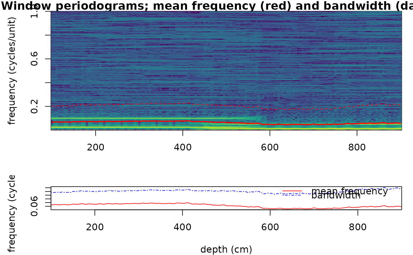
# \donttest{
# Two cycles (40 and 10 cm period in "age" units) recorded with a
# sedimentation rate that doubles halfway the record (depth in cm): the
# mean frequency halves in the upper part.
dt <- 0.5
depth <- seq(0, 1000, by = dt)
age <- ifelse(depth <= 500, depth, 500 + (depth - 500) / 2)
set.seed(1)
proxy <- sin(2 * pi * age / 40) + 0.5 * sin(2 * pi * age / 10) +
  stats::rnorm(length(depth), sd = 0.2)
sm <- spectral_moments(data = cbind(depth, proxy), window = 200,
                       step = 5, pad = 5, genplot = FALSE)
plot_spectral_moments(sm, x_lab = "depth (cm)")


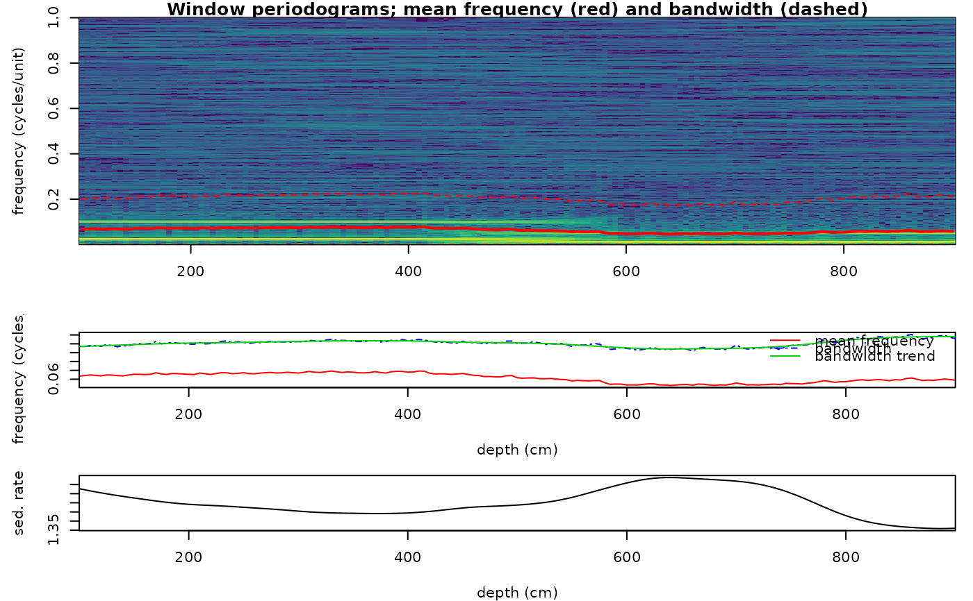
# with a sedimentation-rate estimate (legacy path, 'poly' trend)
sm_sr <- spectral_moments(data = cbind(depth, proxy), window = 200,
                          step = 5, pad = 5, sr_mean = 1.5)
plot_spectral_moments(sm_sr, x_lab = "depth (cm)")

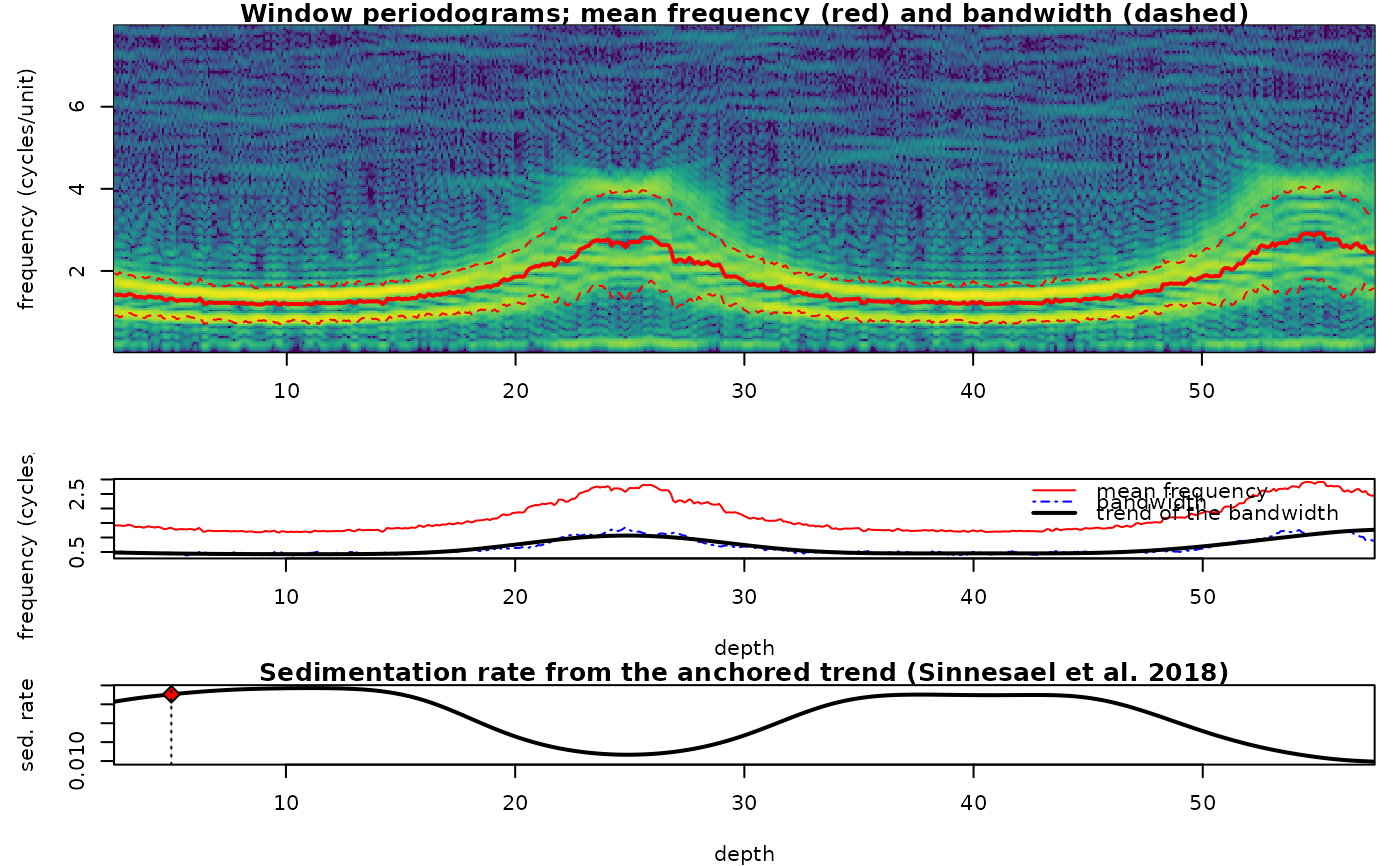
# the sedimentation rate of Sinnesael et al. (2018): the obliquity line is identified at
# 5 m (41 kyr at f_obl cycles/m), the bandwidth trend is anchored there; moments over a band
set.seed(3)
t <- seq(0, 3000, 0.5)
x <- 0.8 * sin(2 * pi * t / 41) + sin(2 * pi * t / 23.7) + 0.5 * sin(2 * pi * t / 405) +
  0.3 * rnorm(length(t))
rate <- 0.02 + 0.01 * sin(2 * pi * t / 1500)
z <- cumsum(c(0, rate[-1] * diff(t)))
zg <- seq(0, max(z), 0.02)
d <- data.frame(zg, approx(z, x, zg)$y)
f_obl <- 1 / (41 * approx(z, rate, 5)$y)     # the obliquity line at 5 m depth
sm <- spectral_moments(d, window = 5, step = 0.1, anchor = c(5, 41, f_obl),
                       freq_range = c(0.1, 8), noise_floor = TRUE)
plot_spectral_moments(sm, freq_max = 8)

# }