The bayes_changepoint function applies the
Bayesian change point algorithm of Ruggieri (2013) to a proxy record. The
record is modelled as a sequence of segments, each described by its own
linear regression (intercept + trend) with conjugate normal /
scaled-inverse-chi-square priors. The algorithm
calculates the marginal likelihood (log form) of every possible sub-interval of the data (Eq. 2 of Ruggieri, 2013),
builds the partition function by forward recursion (dynamic programming, Eqs. 3-4),
calculates the exact posterior distribution of the number of change points (Eqs. 5-7) and
draws
n_simsolutions (number of change points, their locations and the segment regressions) by stochastic backtrace.
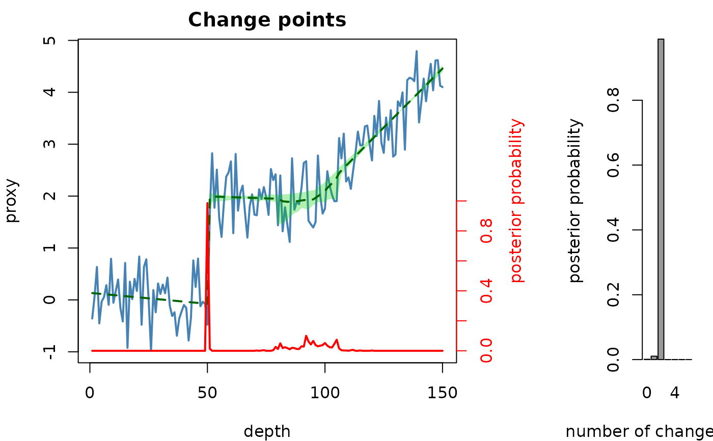
The posterior probability of a change point at each data point, the posterior-mean regression model and its \(R^2\) are returned as in Acycle. In addition the per-sample models are kept, from which pointwise credible intervals of the model are derived (these reflect the uncertainty in the number and location of the change points; each sampled segment uses its posterior-mean regression coefficients, as in Acycle).
Translated from Acycle v3.1 bayes_cpt.m, partition_fn.m, pick_k1.m and nCk.m (Mingsong Li, modified from the code of Eric Ruggieri); default hyperparameters as in the Acycle "Changepoint" menu (AC.m).
Usage
bayes_changepoint(
  data = NULL,
  k_max = 10,
  d_min = 1,
  k_0 = 0.01,
  v_0 = NULL,
  sig_0 = NULL,
  n_sim = 500,
  seed = NULL,
  ci = c(0.025, 0.975),
  stable = FALSE,
  genplot = FALSE,
  verbose = FALSE
)
Arguments
- data
Record to analyse (matrix or data frame with two columns: depth or time in column 1, proxy value in column 2; finite values only, at least two rows). Data points are treated as equally spaced (the regression uses the sample index as predictor, as in Acycle). Required, no default (
Default=NULLgives an error).- k_max
Maximum number of change points considered (integer, >= 1).
Default=10.- d_min
Minimum distance in data points between adjacent change points, i.e. the minimum segment length (integer, >= 1).
Default=1.- k_0
Hyperparameter (variance scaling) of the normal prior on the regression coefficients (numeric, > 0); smaller values give a vaguer prior.
Default=0.01.- v_0
Hyperparameter (number of pseudo data points) of the scaled inverse chi-square prior on the segment variance (numeric, > 0);
NULLusesceiling(abs(x[n] - x[1]) / 44), with x the first column ofdata, as in Acycle.Default=NULL.- sig_0
Hyperparameter (pseudo data variance) of the scaled inverse chi-square prior on the segment variance (numeric, > 0);
NULLuses the variance of the proxy.Default=NULL.- n_sim
Number of solutions (number and positions of the change points with their segment regressions) drawn by stochastic backtrace (integer, >= 1).
Default=500.- seed
Seed of the random number generator (integer), so that the sampled solutions can be reproduced;
NULLleaves the current random state unchanged.Default=NULL.- ci
Lower and upper probabilities of the pointwise credible interval of the model (numeric vector of length 2, between 0 and 1).
Default=c(0.025,0.975).- stable
Use numerically safe log-space arithmetic (shifted log-sum-exp,
lgamma, log binomial coefficients) (logical, TRUE or FALSE). WithFALSEthe arithmetic of Acycle is reproduced exactly (log(sum(exp(.)))in linear space), which under- or overflows for long records or records with a very small or large variance; a warning is given when that happens.Default=FALSE.- genplot
Plot the result with
plot_bayes_changepoint(logical, TRUE or FALSE).Default=FALSE.- verbose
Show a text progress bar while the solutions are sampled (logical, TRUE or FALSE).
Default=FALSE.
Value
A list with elements
model: matrix [x, posterior-mean model] (Acycle "BayesRegModel").cpt: matrix [x, posterior probability of a change point] (Acycle "BayesChangepoint"). A change point at index i means that a new segment starts at index i+1.r2: \(R^2 = 1 - \sum(y-model)^2 / \sum y^2\) as in Acycle.k_posterior: matrix [number of change points (0..k_max), posterior probability].model_ci: matrix [x, lower, median, upper] pointwise credible interval of the sampled models.beta: matrix [intercept, slope] of the posterior-mean regression coefficients at each data point (predictor = sample index).samples:n_simxk_maxmatrix with the index of the sampled change points (0 = none), as Acycle's samp_holder.samples_x: same assamplesexpressed in the unit of the first column (NA = none).n_cpt: sampled number of change points for every solution.sample_models: N xn_simmatrix of the sampled models.log_partition: the k_max x N partition function (log form).param: list with the used hyperparameters.
References
Ruggieri, E. (2013). A Bayesian approach to detecting change points in climatic records. International Journal of Climatology, 33, 520-528. <doi:10.1002/joc.3447>
Li, M., Hinnov, L., Kump, L. (2019). Acycle: Time-series analysis software for paleoclimate research and education. Computers & Geosciences, 127, 12-22. <doi:10.1016/j.cageo.2019.02.011>
Author
Michiel Arts (R translation); original MATLAB code: Eric Ruggieri, modified for Acycle by Mingsong Li.
Examples
# \donttest{
# a record with two changes in mean and one change in trend
set.seed(2)
x <- 1:150
y <- c(rep(0, 50), rep(2, 50), 2 + 0.05 * (1:50)) + stats::rnorm(150, sd = 0.4)
bcp <- bayes_changepoint(data = cbind(x, y), k_max = 6, d_min = 5,
k_0 = 0.01, v_0 = 2, n_sim = 500, seed = 1)
bcp$k_posterior
#> n_changepoints probability
#> [1,] 0 8.762302e-04
#> [2,] 1 1.048529e-02
#> [3,] 2 9.886046e-01
#> [4,] 3 3.387452e-05
#> [5,] 4 1.088208e-09
#> [6,] 5 3.698491e-14
#> [7,] 6 1.456286e-18
plot_bayes_changepoint(bcp)
 # }