Plot the result of bayes_changepoint

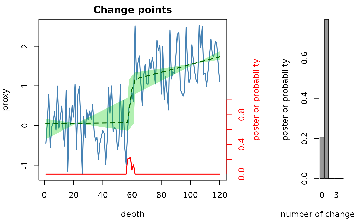
Plots the data, the posterior-mean regression model with its pointwise credible interval, and the posterior probability of a change point (right axis), as in the Acycle change point figure (bayes_cpt.m), together with the posterior distribution of the number of change points.

Usage

plot_bayes_changepoint(
  bcp = NULL,
  x_lab = "depth",
  y_lab = "proxy",
  plot_k = TRUE
)

Arguments

bcp

Change point result to plot: the list returned by bayes_changepoint (its data, model, model_ci, cpt and k_posterior elements are used). Required (Default=NULL gives an error).

x_lab

Label of the depth/time axis (character). Default="depth".

y_lab

Label of the proxy axis (character). Default="proxy".

plot_k

Add a panel to the right with a bar plot of the posterior distribution of the number of change points (logical, TRUE or FALSE). Default=TRUE.

Value

No return value, called for its side effect (a base graphics plot).

References

Ruggieri, E. (2013). A Bayesian approach to detecting change points in climatic records. International Journal of Climatology, 33, 520-528. <doi:10.1002/joc.3447>

Author

Michiel Arts (R translation); original MATLAB code: Eric Ruggieri, Mingsong Li.

Examples

# \donttest{
set.seed(2)
y <- c(rep(0, 60), rep(1.5, 60)) + stats::rnorm(120, sd = 0.5)
bcp <- bayes_changepoint(data = cbind(1:120, y), k_max = 4, d_min = 5,
                         v_0 = 3, n_sim = 200, seed = 1)
plot_bayes_changepoint(bcp)

# }