Cross-validated correlation coefficient (cvCOCO) analysis

The cvcoco function performs the bidirectional held-out ("cross-validated") correlation coefficient (cvCOCO) test of Acycle for astronomical forcing in a depth series. The cleaned record is split into two folds: two contiguous halves at the depth midpoint (method = "blocked", Blocked cvCOCO, the Acycle public default) or the odd and even observations (method = "interleaved", Interleaved cvCOCO). Each fold is linearly interpolated to its own median spacing. In each direction one fold is used for training: at every tested sedimentation rate the energies in four one-Rayleigh union bands (long eccentricity, short eccentricity, obliquity, precession) are leakage-corrected with an exact nonnegative least-squares solve of the finite-record 4x4 leakage matrix, and the rate with the highest spectral correlation gives four trained group amplitudes. These amplitudes are frozen and the held-out fold searches its own sedimentation rate (validation). The same-rate minimum of both directional validation curves is the consensus curve. A single outer stationary AR(1) Monte Carlo reproduces the complete bidirectional train/validate pipeline and gives global (rate-search corrected) and local p-values, the robust directional p-value max(pA, pB) and pCOCO. Two target designs are available: "four-group-coherent-nine" (the four group amplitudes expanded to nine zero-phase sinusoids summed coherently; Acycle cvcoco9B.m / interleavedcvcoco.m, the GUI default) and "four-group" (phase-averaged noncoherent four-group target; Acycle cvcoco2.m, for which Acycle issues the confirmatory conclusion report of cocoConclusionReport.m). The COCO method was introduced by Li et al. (2018). Translated from Acycle v3.1 cvcoco.m, cvcoco2.m, cvcoco9B.m, interleavedcvcoco.m, cocoConclusionReport.m and helpers (Mingsong Li).

This function calls the following helpers of the cocoR port (which must be loaded): coco_orbit_groups, detrend_linear, ml_periodogram and theored_ar1_ml; and, for red = 3, swa_background.

Usage

cvcoco(
  data = NULL,
  orbit9 = c(405.6912, 130.6979, 123.8532, 98.8517, 94.8856, 40.9897, 23.682, 22.3758,
    18.9519),
  pad = 0,
  sr1 = 1,
  sr2 = 20,
  srstep = 0.1,
  red = 0,
  n_sim = 1000,
  cor_method = "Pearson",
  method = "blocked",
  target_model = "four-group-coherent-nine",
  max_frequency = NULL,
  batch_size = 100,
  seed = NULL,
  interleaved_phase = 0,
  genplot = FALSE,
  verbose = FALSE
)

Arguments

data

Record to test (matrix or data frame, two columns): depth in metres in column 1 and the proxy in column 2. Unsorted, duplicated and irregularly spaced depths are allowed (each fold is cleaned and linearly interpolated to its own median spacing). Required (Default=NULL gives an error).

orbit9

The nine astronomical target periods in kyr (numeric vector of nine distinct, positive values): one long eccentricity, four short eccentricity, one obliquity and three precession periods (the groups are identified by descending period rank), e.g. from orbit9_at_age for the age of the record. Default=c(405.6912, 130.6979, 123.8532, 98.8517, 94.8856, 40.9897, 23.6820, 22.3758, 18.9519).

pad

Length (number of points) of the zero-padded periodogram (non-negative integer); each fold uses max(pad, n_fold), so 0 means no padding (as in the Acycle GUI when padding is unchecked); a larger value gives a finer frequency grid but uses more memory. Default=0.

sr1

Lowest sedimentation rate tested, in cm/kyr (numeric, > 0). Default=1.

sr2

Highest sedimentation rate tested, in cm/kyr (numeric, >= sr1). Default=20.

srstep

Step of the sedimentation-rate grid, in cm/kyr (numeric, > 0). Default=0.1.

red

Red-noise background removed from every spectrum (integer): 0 none, 1 classical AR(1), 2 robust AR(1) (median-smoothed spectrum), 3 smoothed-window average (SWA). Default=0.

n_sim

Number of AR(1) Monte Carlo simulations of the complete bidirectional train/validate pipeline, used for the p-values and pCOCO (integer, 0 to 1e6); 0 gives only the deterministic curves. Default=1000.

cor_method

Correlation coefficient used in all spectral correlations (character): "Pearson" or "Spearman". Default="Pearson".

method

How the record is split into the two folds (character): "blocked" (two contiguous halves at the depth midpoint; Blocked cvCOCO, the Acycle default) or "interleaved" (odd and even observations; Interleaved cvCOCO). Default="blocked".

target_model

Design of the target (character): "four-group-coherent-nine" (the four group amplitudes expanded to nine zero-phase sinusoids summed coherently; Acycle GUI default) or "four-group" (phase-averaged, noncoherent four-group target; only allowed with method="blocked"). Default="four-group-coherent-nine".

max_frequency

Highest frequency used in all spectral correlations, in cycles/kyr (numeric, at least the highest orbital frequency max(1/orbit9)); NULL uses 1.2 times the highest orbital frequency. Default=NULL.

batch_size

Number of Monte Carlo realisations processed together (positive integer; it is reduced automatically when memory would run short); larger batches are faster but use more memory. Default=100.

seed

Seed of the random number generator (integer), so that the Monte Carlo results can be reproduced; NULL leaves the current random state unchanged. Default=NULL.

interleaved_phase

Which fold the first cleaned observation belongs to when method="interleaved" (integer): 0 the odd fold, 1 the even fold. Ignored for method="blocked". Default=0.

genplot

Plot the results with plot_cvcoco (logical, TRUE or FALSE). Default=FALSE.

verbose

Print preprocessing information and show a progress bar of the Monte Carlo simulations (logical, TRUE or FALSE). Default=FALSE.

Value

A list with elements name ("Blocked cvCOCO" or "Interleaved cvCOCO"), target_model, sr_grid (tested rates), split_depth, fold_labels, data_clean, data_A, data_B (regularized folds), raw_index_A, raw_index_B, interpolation_A, interpolation_B, sampling_interval_A, sampling_interval_B, train_A, train_B (training curve, best rate, amplitudes, group amplitudes, frozen weights, leakage matrix at best rate), validate_AtoB, validate_BtoA (validation curve, best rate, score, directional p, Wilson interval, global and local p curves, participating periods), consensus (same-rate minimum curve, best rate, global p, p curves, pCOCO curve and maximum), score_symmetric, score_consensus, score_mean, p_sym, p_consensus, p_robust, p_A (B-to-A, fold A held out), p_B (A-to-B, fold B held out), their confidence intervals, p_curve_AtoB, p_curve_BtoA, p_local_curve_AtoB, p_local_curve_BtoA, p_curve_consensus, p_local_curve_consensus, pcoco, null distributions (null_symmetric, null_consensus, null_AtoB, null_BtoA, null_best_rate_AtoB, null_best_rate_BtoA), AR(1) coefficients (rho_A, rho_B, rho_full), geometry diagnostics (orbit_count_A/B, resolved_group_count_A/B, resolved_orbit_mask_A/B, valid_rate_mask_A/B, training_rate_mask_A/B, group_leakage_rcond_A/B, all_nine_rate_range_A/B/shared, active_orbit_count_AtoB/BtoA/ consensus, active_group_count_AtoB/BtoA), degraded_mode, training_completeness, spectra (data and frozen-target temporal spectra at the best rates), n_sim_completed, config, and conclusion (confirmatory report; only for target_model = "four-group", otherwise NULL).

References

Li, M., Kump, L.R., Hinnov, L.A., Mann, M.E., 2018. Tracking variable sedimentation rates and astronomical forcing in Phanerozoic paleoclimate proxy series with evolutionary correlation coefficients and hypothesis testing. Earth and Planetary Science Letters 501, 165-179. doi:10.1016/j.epsl.2018.08.041

Li, M., Hinnov, L., Kump, L., 2019. Acycle: Time-series analysis software for paleoclimate research and education. Computers & Geosciences 127, 12-22. doi:10.1016/j.cageo.2019.02.011

Author

Michiel Arts (R translation); original MATLAB code: Mingsong Li.

Examples

# \donttest{
# synthetic ETP-like series in depth (5 cm/kyr) with AR(1) noise
set.seed(2)
t_kyr <- seq(0, 1600, by = 2)
etp <- sin(2 * pi * t_kyr / 405) + 0.6 * sin(2 * pi * t_kyr / 125) +
  0.5 * sin(2 * pi * t_kyr / 95) + 0.8 * sin(2 * pi * t_kyr / 41) +
  0.5 * sin(2 * pi * t_kyr / 23.7) + 0.4 * sin(2 * pi * t_kyr / 19)
noise <- as.numeric(stats::filter(stats::rnorm(length(t_kyr)), 0.5,
  method = "recursive"))
dat <- cbind(t_kyr * 5 / 100, etp + 0.5 * noise)
res <- cvcoco(data = dat, sr1 = 2, sr2 = 10, srstep = 0.5,
  n_sim = 50, seed = 1)
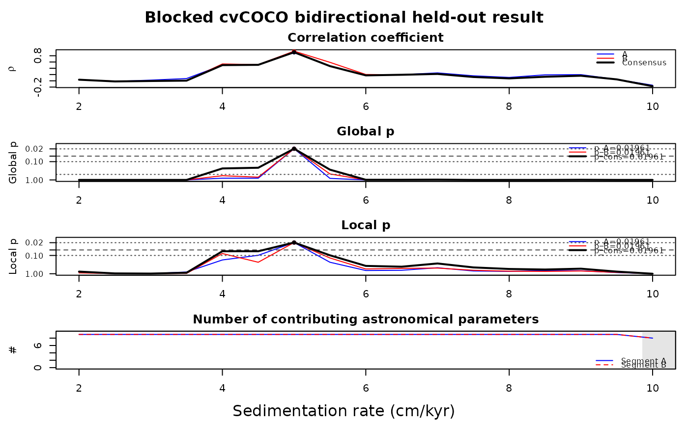
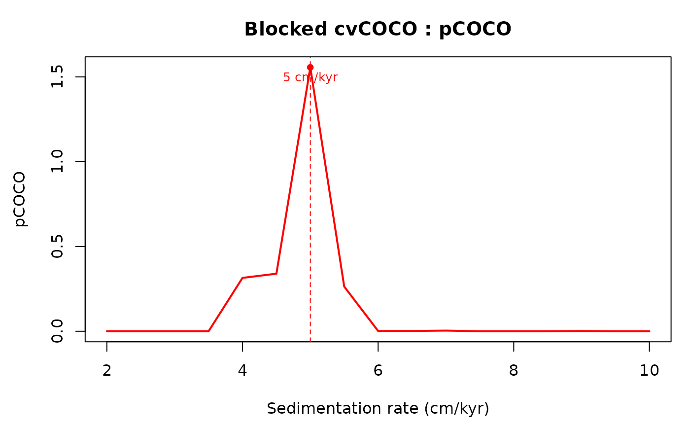
res$consensus$best_rate
#> [1] 5
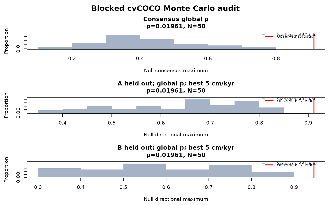
res$p_robust
#> [1] 0.01960784
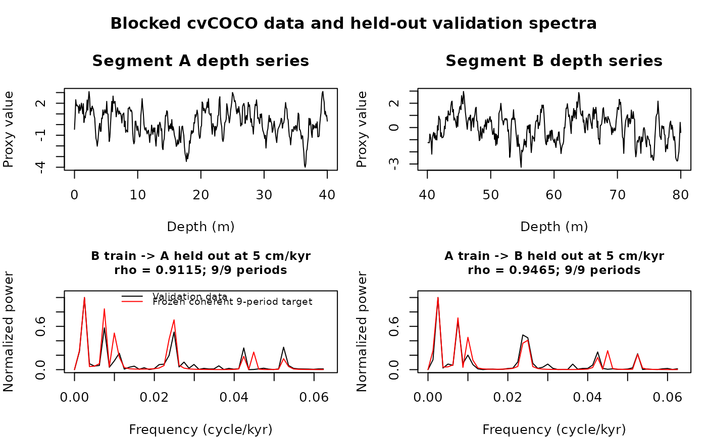
plot_cvcoco(res)




# }