Dynamic (depth-varying) Gaussian band-pass filter — dynamic

The dynamic_filter function extracts a cycle whose frequency changes along the depth/time axis (e.g. because of a changing sedimentation rate) using a pass band that follows user-defined control points. The method is the dynamic filter of Nicolas Thibault and Giovanni Rizzi (2019), adapted by Mingsong Li (2020) for Acycle's "Frequency Stabilization" tool, in the deterministic form of Acycle's current core: the series is divided into sliding windows; in each window the pass band is obtained by linear interpolation of the control points at the window centre (held constant beyond the first/last control point), the window is mean-centred, tapered by the square root of a half-sample-shifted Hann window, Gaussian band-pass filtered (half-power edges at the lower/upper frequency, zero padded to 2^nextpow2(2 * window_samples - 1)), tapered again and overlap-added. The result is divided by the summed Hann weights. In Acycle the control points are clicked on an evolutionary spectrum; here they are supplied as arguments, e.g. built with dynamic_filter_controls from a period curve tracked with WaverideR (track_period_wavelet, completed_series). Translated from Acycle v3.1 acycleDynamicFilter.m (strict core; legacy flow dynamic_filter.m / dynamic_filter_lang.m, GUI DynamicFilter.m) (Mingsong Li).

Usage

dynamic_filter(
  data = NULL,
  controls = NULL,
  window_length = NULL,
  step_length = NULL,
  pad_ends = TRUE,
  genplot = FALSE,
  x_lab = "depth",
  y_lab = "proxy",
  verbose = FALSE
)

Arguments

data

Input series (two-column matrix or data frame of finite numeric values: depth/time in column 1, strictly increasing and regularly sampled to a relative spacing tolerance of 1e-5, proxy value in column 2; at least 8 rows). Interpolate irregular data to a regular grid beforehand. Required (Default=NULL).

controls

Pass band control points, in cycles per depth/time unit. Either

a matrix or data frame with columns depth, f_low, f_high and optionally f_centre (unnamed columns are taken in that order), e.g. the output of dynamic_filter_controls, or
a list with elements lower and upper, each a two-column matrix [depth, frequency] (separate lower/upper boundary picks, which may be at different depths).

Depths must be strictly increasing and lie within the data range, frequencies must be > 0, with f_low < f_high and f_high below the Nyquist frequency everywhere. Between control points the band is linearly interpolated, beyond the first/last point it is held constant; a single row gives a constant pass band. Because the Gaussian response is symmetric, a supplied f_centre must equal (f_low + f_high) / 2 (it is only checked). Required (Default=NULL).

window_length

Length of the sliding windows, in depth/time units (numeric, > 0, at most the record length and at least 8 samples). Longer windows give a sharper frequency resolution but follow changes in the pass band less closely; a window of about two times the longest period of the target cycle is recommended. NULL uses 20% of the record length (Acycle GUI default). Default=NULL.

step_length

Step between successive windows, in depth/time units (numeric, > 0, between half a sample interval and window_length). NULL uses 4 times the sample interval, or (record length - window_length) / 500 when that would give more than 500 steps (Acycle GUI default). Default=NULL.

pad_ends

Mirror the record at both ends by one window length before filtering (logical, TRUE or FALSE). The first and last samples are then covered by many windows; without padding they are covered by a single window whose taper weight is close to zero, and dividing by that weight inflates the filtered values at the ends. FALSE reproduces Acycle exactly. Default=TRUE.

genplot

Plot the data and the filtered signal with plot_dynamic_filter (logical, TRUE or FALSE). Default=FALSE.

x_lab

Label of the depth/time axis of the plot, passed to plot_dynamic_filter (character). Only used when genplot=TRUE. Default="depth".

y_lab

Label of the proxy axis of the plot, passed to plot_dynamic_filter (character). Only used when genplot=TRUE. Default="proxy".

verbose

Show a progress bar over the windows (logical, TRUE or FALSE). Default=FALSE.

Value

A list with elements

filtered: matrix with columns depth, filtered, coverage_count (number of windows covering each sample) and coverage_weight (sum of Hann weights).
windows: matrix with one row per window and columns centre, f_low, f_high, f_centre, start_depth, end_depth, start_index, end_index.
lower_controls, upper_controls: the 2-column [depth, frequency] control points used.
sample_interval: median sample spacing.
nyquist: Nyquist frequency.
window_samples, step_samples: window and step in samples.
window_length, step_length: effective (sample-rounded) window and step in depth units.
fft_length: zero-padded FFT length per window.
terminal_window_appended: whether a final window ending on the last sample was added.

References

Li, M., Hinnov, L., Kump, L., 2019. Acycle: Time-series analysis software for paleoclimate research and education. Computers & Geosciences 127, 12-22. <doi:10.1016/j.cageo.2019.02.011>

Thibault, N., Rizzi, G. (2019). Dynamic filtering routine, distributed with Acycle (Frequency Stabilization).

Author

Michiel Arts (R translation); original MATLAB code: Nicolas Thibault and Giovanni Rizzi (2019), adapted by Mingsong Li (Acycle).

Examples

# \donttest{
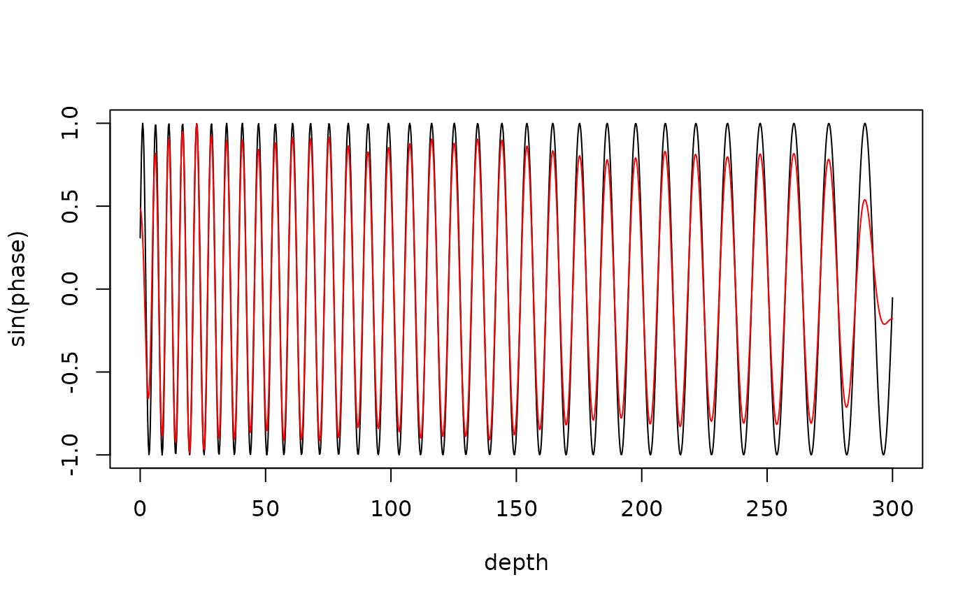
# cycle whose period grows linearly from 5 to 15 m (changing sed. rate)
depth <- seq(0, 300, by = 0.25)
period <- 5 + 10 * depth / 300
phase <- 2 * pi * cumsum(1 / period) * 0.25
set.seed(1)
proxy <- sin(phase) + 0.8 * sin(2 * pi * depth / 2.1) + rnorm(length(depth), sd = 0.3)
ctrl <- dynamic_filter_controls(tracked = cbind(depth, period),
  rel_bandwidth = 0.3, n_points = 30)
res <- dynamic_filter(data = cbind(depth, proxy), controls = ctrl,
  window_length = 40, step_length = 1, genplot = FALSE)
plot(depth, sin(phase), type = "l")
lines(res$filtered[, 1], res$filtered[, 2], col = "red")

# }