Plot the result of a dynamic filter

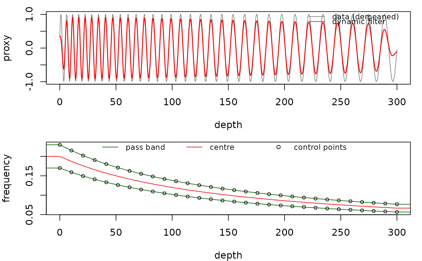
The plot_dynamic_filter function plots the output of dynamic_filter: the (demeaned) data with the filtered signal, and the depth-varying pass band (window lower, upper and centre frequencies or periods, with the control points), reproducing the overlay Acycle draws on its evolutionary spectrum (dynamic_filter_lang.m). Written for the R translation of Acycle v3.1 dynamic filtering (Mingsong Li).

Usage

plot_dynamic_filter(
  data = NULL,
  dyn_filter = NULL,
  period = FALSE,
  x_lab = "depth",
  y_lab = "proxy"
)

Arguments

data

Record that was filtered, the same as given to dynamic_filter: a two-column matrix or data frame with depth/time in column 1 and the proxy value in column 2. It is drawn demeaned in the top panel. Required (Default=NULL gives an error).

dyn_filter

Dynamic filter result to plot: the list returned by dynamic_filter (its filtered, windows, lower_controls and upper_controls elements are used). Required (Default=NULL gives an error).

period

Unit of the pass band in the bottom panel (logical): TRUE draws the band limits, centre and control points as periods (1/frequency, depth/time units), FALSE as frequencies (cycles per depth/time unit). Default=FALSE.

x_lab

Label of the depth/time axis of both panels (character). Default="depth".

y_lab

Label of the y-axis of the data panel (character). Default="proxy".

Value

No return value; a plot is produced.

References

Li, M., Hinnov, L., Kump, L., 2019. Acycle: Time-series analysis software for paleoclimate research and education. Computers & Geosciences 127, 12-22. <doi:10.1016/j.cageo.2019.02.011>

Author

Michiel Arts (R translation); original MATLAB code: Nicolas Thibault, Giovanni Rizzi and Mingsong Li (Acycle).

Examples

# \donttest{
depth <- seq(0, 300, by = 0.25)
period <- 5 + 10 * depth / 300
proxy <- sin(2 * pi * cumsum(1 / period) * 0.25)
ctrl <- dynamic_filter_controls(tracked = cbind(depth, period),
  rel_bandwidth = 0.3, n_points = 30)
res <- dynamic_filter(data = cbind(depth, proxy), controls = ctrl,
  window_length = 40, step_length = 1)
plot_dynamic_filter(data = cbind(depth, proxy), dyn_filter = res)

# }