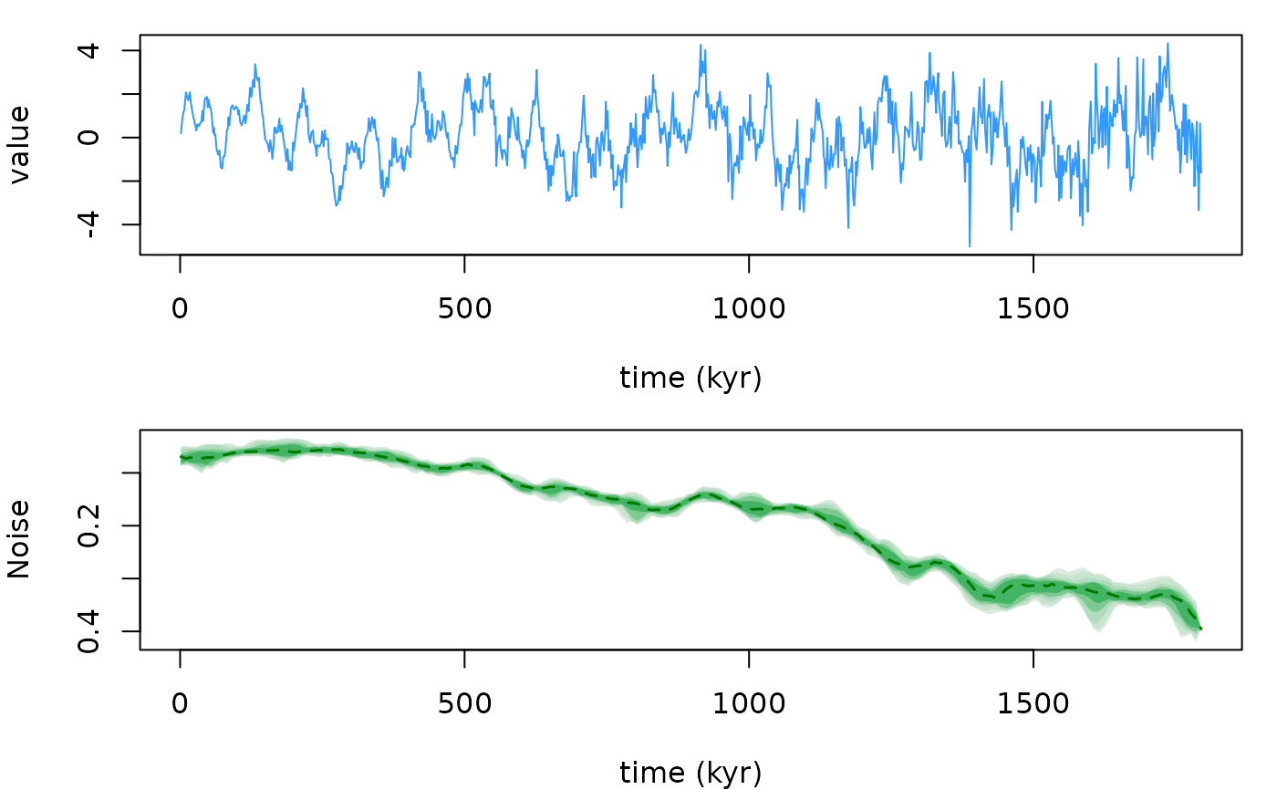
The dynot function runs the DYNOT sedimentary
noise model of Li et al. (2018a,b) on an (orbitally tuned, usually
unevenly sampled) time series. In each Monte Carlo realisation a sampling
interval is drawn from a Weibull distribution fitted (maximum likelihood)
to the sampling intervals of the data (values outside
[sample_min, sample_max] are replaced by one shared uniform
draw for all low values and one for all high values, as in Acycle), a
window length is drawn uniformly from [window_min, window_max],
a time-bandwidth product from nw_min + k/2 and, for each target
orbital frequency f, the lower and upper band limits are
f -/+ fz * nw / window with fz uniform in [fz_min, fz_max].
The series is pchip-interpolated at the drawn sampling interval, linearly
detrended, padded by half a window (pad_type) and analysed with the
legacy power decomposition (pdan.m, see pda_legacy).
The power-ratio curves are interpolated onto a regular grid, rescaled by
(grand mean / realisation mean) of the power ratio, normalised to a
maximum of 1 if needed, and summarized by percentiles (median plus the
selected confidence intervals). The noise is 1 - power ratio.
Translated from Acycle v3.1 DYNOS.m (runDynot, loadDataReady,
sanitizeData), dynotIterationWorker.m, dynotPercentilePlan.m, pdan.m and
zeropad2.m (Mingsong Li).
Usage
dynot(
  data = NULL,
  target_periods = c(405.6912, 130.6979, 123.8532, 98.8517, 94.8856, 40.9897, 23.682,
    22.3758, 18.9519),
  window_min = 300,
  window_max = 500,
  nw_min = 2,
  nw_max = 2,
  pad = 1000,
  step = 5,
  n_out = 1000,
  pad_type = 1,
  fz_min = 0.9,
  fz_max = 1.2,
  f_min = 0.001,
  f_max = 1,
  sample_min = NULL,
  sample_max = NULL,
  intervals = c(50, 68, 80, 90, 95),
  n_sim = 1000,
  seed = NULL,
  verbose = FALSE,
  genplot = FALSE
)
Arguments
- data
Tuned time series (matrix or data frame, numeric: time in column 1, e.g. in kyr, proxy value in column 2; further columns are ignored; at least 10 rows; may be unevenly sampled). Rows are sorted, duplicated times are averaged and non-finite rows removed. Required (
Default=NULL).- target_periods
Periods of the target orbital cycles, in the time unit of
data(numeric vector, > 0). The power within a band around each target frequency1 / periodis summed into the target power.Default=c(405.6912, 130.6979, 123.8532, 98.8517, 94.8856, 40.9897, 23.6820, 22.3758, 18.9519)(the nine Acycle default periods in kyr).- window_min, window_max
Range of the sliding window length, in the time unit of
data(numeric, > 0,window_min <= window_max); each Monte Carlo realisation draws its window length uniformly from this range.Default=300andDefault=500.- nw_min
Smallest time-bandwidth product of the multitaper spectra (numeric, >= 0.5). Each realisation uses
nw_min + k/2, withkdrawn from1:(2*(nw_max-nw_min)), ornw_minitself whennw_max=nw_min.Default=2.- nw_max
Largest time-bandwidth product (numeric, >=
nw_min);2*(nw_max-nw_min)must be an integer. If equal tonw_min, all realisations usenw_min.Default=2.- pad
Number of points (zero-padded FFT length) of each multitaper spectrum (integer, > 0); larger values give a finer frequency grid.
Default=1000.- step
Step between successive windows of the power decomposition, in samples of the interpolated series (integer, >= 1).
Default=5.- n_out
Number of points of the regular output time grid onto which the noise curves are interpolated (integer, >= 1).
Default=1000.- pad_type
How the series is extended by half a window at both ends before the analysis (numeric code):
0no padding,1zeros,2mirrored data,3the mean of the end segment,4random normal values with the mean and standard deviation of the end segment.Default=1.- fz_min, fz_max
Range of the bandwidth multiplier (numeric, > 0,
fz_min <= fz_max): the lower and upper limits of each target band aref -/+ fz * nw / window, withfzdrawn uniformly from this range for each limit and realisation.Default=0.9andDefault=1.2.- f_min
Lower frequency limit, in cycles per time unit (numeric, >= 0): target band limits below it are clipped to it and it is the lower edge of the total band used as denominator of the power ratio.
Default=0.001.- f_max
Upper frequency limit, in cycles per time unit (numeric, >
f_min): target band limits above it are clipped and it is the upper edge of the total band (itself clipped to the Nyquist frequency).Default=1.- sample_min
Smallest simulated sampling interval, in the time unit (numeric, > 0, or
NULL). Each realisation interpolates the series to a sampling interval drawn from a Weibull distribution fitted to the sampling intervals ofdata; draws belowsample_minare replaced by one shared uniform draw from [sample_min,sample_max].NULLuses the 5th percentile of the data sampling intervals.Default=NULL.- sample_max
Largest simulated sampling interval (numeric, >=
sample_min, orNULL); draws above it are replaced in the same way.NULLuses the 95th percentile of the data sampling intervals.Default=NULL.- intervals
Confidence intervals of the noise to report, in percent (numeric vector, any subset of
50,68,80,90,95); the median is always reported.Default=c(50, 68, 80, 90, 95).- n_sim
Number of Monte Carlo realisations (integer, >= 1).
Default=1000.- seed
Seed of the random number generator (integer), so that the Monte Carlo results can be reproduced;
NULLleaves the current random state unchanged.Default=NULL.- verbose
Show a progress bar over the realisations (logical, TRUE or FALSE).
Default=FALSE.- genplot
Plot the result with
plot_dynot(logical, TRUE or FALSE).Default=FALSE.
Value
A list with elements
percentile: matrix [time, noise percentiles] on the grid points
where the median is defined (column names give the percentile levels);
median: matrix [time, median noise];
percentiles: percentile levels; median_index;
interval_count: number of confidence intervals;
grid: full output grid; noise: matrix (n_out x n_sim) of
adjusted noise (1 - adjusted power ratio) of every realisation;
power_mean: mean power ratio of every realisation;
draws: list with the simulated sampling intervals, windows, nw,
band limits (matrix f3m) and the underlying uniform draws;
weibull: fitted Weibull scale and shape; sample_range;
data: the cleaned input data.
References
Li, M., Hinnov, L.A., Huang, C., Ogg, J.G., 2018a. Sedimentary noise and sea levels linked to land-ocean water exchange and obliquity forcing. Nature Communications 9, 1004. doi:10.1038/s41467-018-03454-y
Li, M., Huang, C., Hinnov, L., Chen, W., Ogg, J., Tian, W., 2018b. Astrochronology of the Anisian stage (Middle Triassic) at the Guandao reference section, South China. Earth and Planetary Science Letters 482, 591-606. doi:10.1016/j.epsl.2017.11.042
Li, M., Huang, C., Hinnov, L., Ogg, J., Chen, Z.-Q., Zhang, Y., 2016. Obliquity-forced climate during the Early Triassic hothouse in China. Geology 44, 623-626. doi:10.1130/G37970.1