Continuous tracking of a cycle in a (synchrosqueezed) scalogram with a hidden Markov model

Tracks the period of one cycle continuously through a scalogram made by analyse_wavelet, analyse_wavelet_sst, analyse_superlet_sst, analyse_conceft or any object of class analyze.wavelet. Sharp synchrosqueezed scalograms can have gaps where the cycle is weak (low eccentricity, noise, a facies change), which makes manual or ridge-by-ridge tracking discontinuous. Here the period at every position is a hidden state that follows a random walk (the sedimentation rate changes gradually, with an optional small probability of an abrupt change, e.g. at a hiatus) and the scalogram is the evidence. 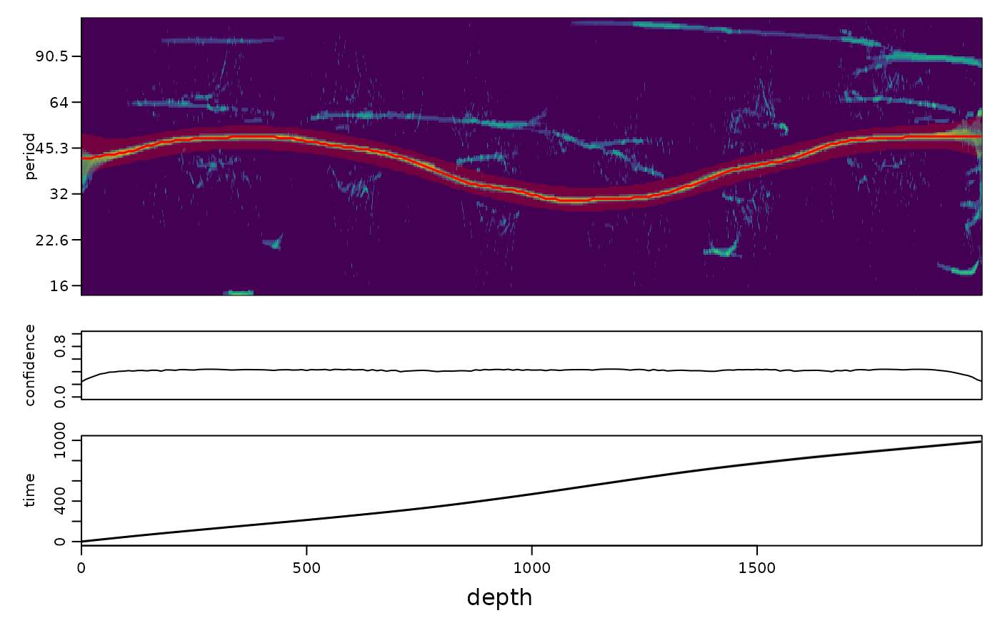The forward-backward algorithm combines the evidence of the whole record: where the cycle is clear it fixes the period, and through gaps the track is bridged by the neighbouring evidence and by the fallback scalogram (the ordinary wavelet power, which is never empty). The result is a continuous curve with

the most probable path (Viterbi),
the posterior mean and a credible band of the period at every position,
a confidence value (the posterior probability within 2 percent of the tracked period), which shows where the track is constrained by data and where it is interpolated,
optionally (period_of_tracked_cycle) the sedimentation rate and an age model with uncertainty from paths sampled from the posterior.

The first two columns (depth, period) can be used directly by curve2time and the other functions that take a tracked curve.

Usage

track_ridge_hmm(
  wavelet,
  period = NULL,
  guide = NULL,
  guide_tolerance = 0.25,
  sd_change = 0.1,
  jump_prob = 0.001,
  smooth_period = 0.02,
  smooth_depth = NULL,
  fallback = "cwt",
  fallback_weight = 0.2,
  sharpness = 0.5,
  n_positions = 1500,
  period_of_tracked_cycle = NULL,
  n_samples = 200,
  level = 0.95,
  jump_depths = NULL,
  constraints = NULL,
  jump_prob_at = 0.05,
  seed = 1
)

Arguments

wavelet: Scalogram to track (list of class analyze.wavelet), the output of analyse_wavelet, analyse_wavelet_sst, analyse_superlet_sst, analyse_conceft or a similar function; its elements Power, Period, axis.1, dt, dj, x and y are used. Required, no default.
period: Period band in which the cycle is searched (numeric vector c(lower, upper), in the depth/time unit of the record; must hold at least three periods of the scalogram). Either period or guide must be given; with a guide the band is taken from the guide instead. Default=NULL.
guide: Optional rough track of the cycle (two-column data frame or matrix: depth in column 1, period in column 2, in depth units), e.g. from track_period_wavelet or a previous run. It is interpolated to all positions (constant beyond its ends) and the search is restricted to guide * (1 +- guide_tolerance); NULL uses period only. Default=NULL.
guide_tolerance: Relative half width of the search band around guide (numeric, > 0; e.g. 0.25 allows periods from 0.8 to 1.25 times the guide). Default=0.25.
sd_change: Standard deviation of the change of log2(period) over a distance of one period (numeric, > 0); it sets how smoothly the track may wander. 0.1 is about 7 percent per cycle; larger values follow faster changes of the sedimentation rate, smaller values give a smoother track. Default=0.1.
jump_prob: Probability of an abrupt change of the period (a jump to any period of the band) between neighbouring positions of the track (numeric, between 0 and 1). Default=1e-3.
smooth_period: Gaussian smoothing of the scalogram along the period axis before tracking (numeric, >= 0; the standard deviation in octaves; 0 switches it off). Default=0.02.
smooth_depth: Width of the moving average of the scalogram along the record before tracking (numeric, in depth units, >= 0); NULL uses the lower limit of the band (one shortest period). Default=NULL.
fallback: Second source of evidence that is mixed in where the scalogram is empty (sharp synchrosqueezed maps): "cwt" the normalised Morlet wavelet power (the element Power_cwt of wavelet if present, otherwise computed with analyse_wavelet, omega_nr = 8), another scalogram object (list with a Power matrix on the same grid as wavelet), or "none" (no fallback). Default="cwt".
fallback_weight: Weight of the fallback evidence in the mix (numeric, between 0 and 1; the scalogram gets 1 - fallback_weight); 0 switches the fallback off. Default=0.2.
sharpness: Weight of the evidence relative to the smoothness of the track (numeric, > 0). Because neighbouring positions of a scalogram are not independent, the log evidence is scaled so that one period of the cycle counts as one observation; larger values trust the scalogram more and give narrower credible bands; with 0.5 the 95 percent bands of the age model contained the true age 95 to 100 percent of the time in synthetic tests. Default=0.5.
n_positions: Maximum number of positions along the record at which the track is computed (integer, > 1); the result is interpolated to all positions of the scalogram. Fewer positions are used when they would be closer than a quarter of the (geometric mean) period of the band. Default=1500.
period_of_tracked_cycle: Optional duration of the tracked cycle in time units (numeric, e.g. 405 for the 405-kyr eccentricity cycle). If given, the sedimentation rate (period / period_of_tracked_cycle) and an age model with uncertainty from posterior paths are added; it is required for constraints; NULL returns only the period track. Default=NULL.
n_samples: Number of paths drawn from the posterior to compute the uncertainty of the sedimentation rate and of the age model (integer, >= 1); only used with period_of_tracked_cycle. Default=200.
level: Probability content of the credible bands (numeric, between 0 and 1, e.g. 0.95 for the 2.5 to 97.5 percent quantiles). Default=0.95.
jump_depths: Optional depths where an abrupt change of the sedimentation rate is plausible (numeric vector, in depth units): a hiatus, erosion surface, abrupt facies change or tectonic contact known from the field or from a change-point analysis such as bayes_changepoint. Within 1.5 track steps of these depths the jump probability is raised to jump_prob_at. Abrupt changes are hard to detect from the scalogram alone in noisy records, so giving them helps the track to follow the jump instead of smoothing it. Default=NULL (none).
constraints: Optional geological duration constraints (data frame, one row per constraint; the first three columns are read as from, to (depths) and duration (time, in the unit of period_of_tracked_cycle, e.g. kyr); an optional column tolerance gives the allowed relative deviation, default 0.025), for instance a biostratigraphic bracket, the time between two dated ash beds or the duration of a stage known from another section. Intervals must not overlap. Needs period_of_tracked_cycle. The track is then the most probable one that satisfies them: the evidence is tilted by a Lagrange multiplier times the time spent in each interval, with the multiplier found by bisection so that the interval has the required duration. The achieved durations and multipliers are returned in the attribute constraints. Default=NULL (none).
jump_prob_at: Jump probability between neighbouring positions near jump_depths (numeric, between 0 and 1; replaces jump_prob there if larger). Default=0.05.
seed: Seed of the random number generator for the posterior sampling (integer), so that the credible bands of the age model can be reproduced; the random state of the session is restored afterwards. Default=1.

Value

A data frame of class wr_track with the columns depth, period (Viterbi path), period_mean, period_lower, period_upper, confidence and, with period_of_tracked_cycle, sedrate (depth units per time unit), sedrate_lower, sedrate_upper, time, time_lower and time_upper (time since the top/start of the record).

References

Rabiner, L.R., 1989. A tutorial on hidden Markov models and selected applications in speech recognition. Proceedings of the IEEE 77, 257-286.

Carmona, R.A., Hwang, W.L., Torresani, B., 1997. Characterization of signals by the ridges of their wavelet transforms. IEEE Transactions on Signal Processing 45, 2586-2590.

Examples

# \donttest{
set.seed(1)
z <- 0:1999
Pt <- 40 + 10 * sin(2 * pi * z / 1500)
amp <- 0.3 + abs(sin(2 * pi * z / 600))
x <- amp * sin(2 * pi * cumsum(1 / Pt)) + rnorm(length(z), sd = 0.5)
s <- analyse_superlet_sst(data.frame(z, x), lowerPeriod = 15, upperPeriod = 120, dj = 1 / 50)
tr <- track_ridge_hmm(s, period = c(25, 70), period_of_tracked_cycle = 20)
plot_track(tr, s)

# }