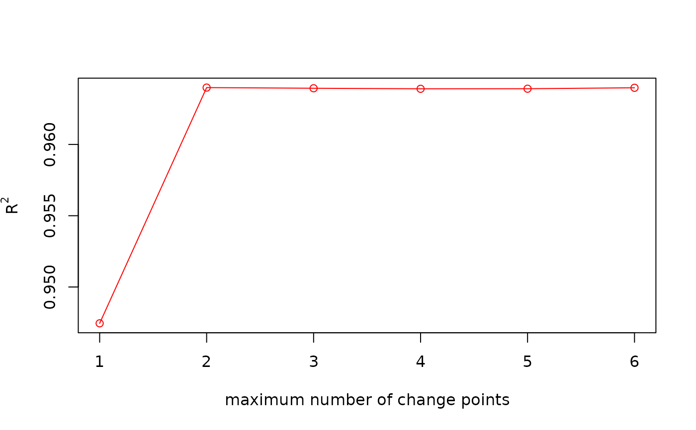
R-squared of the Bayesian change point model as a function of the maximum number of change points

The bayes_changepoint_r2 function runs the Bayesian change point algorithm of Ruggieri (2013) (see bayes_changepoint) for a maximum number of change points k = 1, 2, ..., k_max and returns the \(R^2\) of the posterior-mean model for each k. This helps to choose k_max. Translated from Acycle v3.1 bayes_cpt_r2.m (Mingsong Li, modified from the code of Eric Ruggieri). Note: the Acycle code loops over k but always uses the full k_max inside the loop (the loop index is unused), so it returns k_max replicate R2 values of the same model; here the loop index is used as the maximum number of change points, as intended. The sub-interval likelihoods and the partition function are calculated once (the rows of the partition function do not depend on k_max).

Usage

bayes_changepoint_r2(
  data = NULL,
  k_max = 10,
  d_min = 1,
  k_0 = 0.01,
  v_0 = NULL,
  sig_0 = NULL,
  n_sim = 500,
  seed = NULL,
  stable = FALSE,
  genplot = FALSE,
  verbose = FALSE
)

Arguments

data

Record to analyse (matrix or data frame with two columns: depth or time in column 1, proxy value in column 2; finite values only, at least two rows). Data points are treated as equally spaced (the regression uses the sample index as predictor, as in Acycle). Required, no default (Default=NULL gives an error).

k_max

Maximum number of change points considered (integer, >= 1). Default=10.

d_min

Minimum distance in data points between adjacent change points, i.e. the minimum segment length (integer, >= 1). Default=1.

k_0

Hyperparameter (variance scaling) of the normal prior on the regression coefficients (numeric, > 0); smaller values give a vaguer prior. Default=0.01.

v_0

Hyperparameter (number of pseudo data points) of the scaled inverse chi-square prior on the segment variance (numeric, > 0); NULL uses ceiling(abs(x[n] - x[1]) / 44), with x the first column of data, as in Acycle. Default=NULL.

sig_0

Hyperparameter (pseudo data variance) of the scaled inverse chi-square prior on the segment variance (numeric, > 0); NULL uses the variance of the proxy. Default=NULL.

n_sim

Number of solutions (number and positions of the change points with their segment regressions) drawn by stochastic backtrace (integer, >= 1). Default=500.

seed

Seed of the random number generator (integer), so that the sampled solutions can be reproduced; NULL leaves the current random state unchanged. Default=NULL.

stable

Use numerically safe log-space arithmetic (shifted log-sum-exp, lgamma, log binomial coefficients) (logical, TRUE or FALSE). With FALSE the arithmetic of Acycle is reproduced exactly (log(sum(exp(.))) in linear space), which under- or overflows for long records or records with a very small or large variance; a warning is given when that happens. Default=FALSE.

genplot

Plot the result with plot_bayes_changepoint (logical, TRUE or FALSE). Default=FALSE.

verbose

Show a text progress bar while the solutions are sampled (logical, TRUE or FALSE). Default=FALSE.

Value

A matrix with columns k_max and r2.

References

Ruggieri, E. (2013). A Bayesian approach to detecting change points in climatic records. International Journal of Climatology, 33, 520-528. <doi:10.1002/joc.3447>

Author

Michiel Arts (R translation); original MATLAB code: Eric Ruggieri, modified for Acycle by Mingsong Li.

Examples

# \donttest{
set.seed(2)
x <- 1:150
y <- c(rep(0, 50), rep(2, 50), 2 + 0.05 * (1:50)) + stats::rnorm(150, sd = 0.4)
r2 <- bayes_changepoint_r2(data = cbind(x, y), k_max = 6, d_min = 5,
                           v_0 = 2, n_sim = 200, seed = 1, genplot = TRUE)

# }